– Sets and subsets
– Power set
– Common notations
– How to specify a set
Lecture 2
– The penny problem
– Set operations: union, intersection, difference and complement
– Disjoint sets
– Venn diagram
– (A \cup B)^c = A^c \cap B^c
Lecture 3
– Cardinality
– Inclusion–exclusion principle
– Cartesian plane and cartesian product
– Notation for intervals
– Functions: definition, domain, codomain and image
– Graph representation
– Absolute value
– Bounded functions
Lecture 4
– Injective, surjective and bijective functions
– Composition of functions
– Invertible functions
– Equivalence between invertible and bijective functions
Lecture 5
– Invertible functions (continuation)
– Example of how to find the inverse of a function
– Example where (f \circ g)(x) = x does not imply (g \circ f)(x) = x
– Triangle inequality
– MA-MG inequality
– Definition of statement/proposition
Lecture 6
– Negation
– Logical operators: conjunction, disjunction, conditional and biconditional
– Truth tables
– Compound propositions
– Tautology and contradiction
– Propositional equivalence
– De Morgan laws and other useful equivalence laws
Lecture 7
– Satisfiability and solutions
– Predicate logic (definitons of subject and predicate)
– Quantifiers (universal and existential)
Lecture 8
– Negation of quantified expressions
– Nested quantifiers
– Elementary methods of proof: direct proof, contrapositive and contradiction
– Observation on algebraic manipulations
– Definition of converse
– Proof strategy: looking for invariants
Lecture 9
– Peano’s axioms
– Definition of sum
– Definition of product
– Associativity, distributivity, comutativity and cancellation law
Lecture 10
– Proof of the cancellation law
– Definition of order in \mathbb{N}
– Facts about order
– The well-ordering principle
Lecture 11
– The well-ordering principle is equivalent to the induction axiom
– Strong induction is equivalent to weak induction
– For every n \in \mathbb{N}, we have 1 + \dfrac{1}{2} + \ldots + \dfrac{1}{n} \ge 1 + \dfrac{n}{2}
– For every n \in \mathbb{N}, we have 3 \vert (n^3 - n)
Lecture 12
Applications of induction:
– Sum of the first n natural numbers
– Sum of the first n odd numbers
– Fundamental theorem of arithmetic (existence)
– Let n be the nth Fibonacci number. Then, f_n > \alpha^{n-2}, where \alpha is the golden ration.
Lecture 13
– Solving questions of the mock exam
Lecture 14
This lecture was based on the following notes: construction-of-Q-and-Z
Be careful when you read it. There are some tiny mistakes.
They also defined the set \mathbb{N} containing the element 0. We don’t.
Some small adaptations are necessary to make everything work when \mathbb{N} does not contain 0.
You can find these adaptations explicitly in my notes.
– Equivalence relation
– Equivalence classes
– Proof that equivalence classes partition sets
– Definition of \mathbb{Z} using an equivalence relation in \mathbb{N} \times \mathbb{N}
– How to add, multiply and order in \mathbb{Z}
Lecture 15
– Definition of \mathbb{Q} using an equivalence relation in \mathbb{Z} \times \mathbb{N}
– Proof that we indeed have a well-defined equivalence relation
– How to add, multiply and order in \mathbb{Q}
– Existence of multiplicative inverses
– Archimedean property
Lecture 16
– Method of descent
– The equation x^2 = 2 does not have any rational solutions
– Definition of sequence
– Definition of convergence to a limit in \mathbb{Q} and examples
– Definition of Cauchy sequence and examples
Lecture 17
– Every Cauchy sequence is bounded
– Definition 3.1: equivalence relation
– Theorem 3.2: equivalence classes are either equal or disjoint
– Corollary 3.3: equivalence classes partition the ground set
– Definition 4.1: equivalence relation among Cauchy sequences
– Proposition 4.2: the relation defined in 4.1 is indeed an equivalence relation
Lecture 18
– Definition 4.3: definition of real numbers
– Definition 4.4: embedding the rational numbers into the real numbers
– Definition 4.5: sum and product of real numbers
– Proposition 4.6: sum and product in \mathbb{R} are well-defined
– Lemma 4.8: every Cauchy sequence which is not in the equivalence class of 0 is ‘far’ from 0 after a certain point
Lecture 19
– Theorem 4.7: every real number different from 0 admits a multiplicative inverse
– Definition 4.9: order in the real numbers
– Theorem 4.11: \mathbb{R} has the archimedean property
Lecture 20
– Theorem 4.12: \mathbb{Q} is dense in \mathbb{R}
– Let (x_n)_{n \in \mathbb{N}} be a non-decreasing and bounded sequence. Then, (x_n)_{n \in \mathbb{N}} is Cauchy. A proof of this can be found here.
– Lemma 4.14: the upper bound sequence (u_n)_{n \in \mathbb{N}} is non-increasing and the lower bound sequence (\ell_n)_{n \in \mathbb{N}} is non-decreasing
Lecture 21
– Theorem 4.13: \mathbb{R} has the least upper bound property
– Pigeonhole principle and introduction to Bolzano–Weierstrass. A proof can be found here.
Lecture 22
– Recalling the definition of convergent sequence: page 259, def 13.10.
– Recalling the definition of infimum and supremum: page 256, def 13.3
– Monotone convergence theorem: page 261, thm 13.16
– Limits and arithmetic: page 272, thm 14.5
Lecture 23
– Existence of \sqrt{2}: page 257, example 13.7
– Every convergent sequence has a unique limit: page 260, Lemma 13.14
– If a_n \to L and b_n - a_n \to 0, then b_n \to L: page 272, Lemma 14.3
-If a_n \to 0 and (b_n)_n is bounded, then a_nb_n \to 0 : page 274, Proposition 14.7
– The squeeze theorem: suppose that a_n \le b_n \le c_n for all n \in \mathbb{N} . If a_n \to L and c_n \to L, then also b_n \to L. Page 273, Theorem 14.6
– Bolzano–Weiestrass theorem: every bounded sequence of real numbers has a convergent subsequence. Page 277, Theorem 14.17.
Lecture 24
– Solution of the problems in the mock exam.
Lecture 25
– Theorem 14.19, page 279: Every Cauchy sequence is convergent.
– Definition 14.20, page 279: convergent series.
– Lemma 14.27, page 281: If \sum a_k converges, then a_k \to 0.
– Recalling that the harmonic series is an example where the terms tend to 0 but the series diverges (Example 14.28, page 282)
– Proposition 14.10, page 275: If (b_n)_n is a sequence such that |b_{n+1}/b_n| \to x, where x \in [0,1), then b_n \to 0.
– Theorem 14.24, page 280: \sum_{i=0}^{\infty} \beta^n = (1-\beta)^{-1} if |\beta|<1 .
Lecture 26
– Proposition 14.29, page 282: The comparison test.
– Corollary 14.30, page 283: if \sum |a_k| converges, then \sum a_k converges.
– Theorem 14.31, page 283: The ratio test.
– Example 14.32, page 284: Exponential series.
– Theorem 14.33, page 284: Root test.
Lecture 27
– Definition of deleted neighborhood, page 294
– Definition 15.4, page 294: \lim \limits_{x \to a} f(x)
– Definition 15.7, page 295: sequential limit
– Theorem 15.8, page 295: equivalence between sequential limit and limit
– Lemma 15.9, page 296: limit of sum and product of functions
– Definition 15.10, page 296: continuous functions
– Examples of non-continuous functions in one point and in all points
– Example of continuous functions: polynomials
– Proposition 15.13, page 297: squeeze theorem for continuity
Lecture 28
– Theorem 15.16, page 298: Continuity of composite functions
– Theorem 15.19, page 299: The intermediate value theorem
– Corollary 15.21, page 300: if f:[0,1]\to [0,1] is a continuous function, then it has a fixed point.
– Theorem 15.24, page 302: if f is continuous in a closed interval, then it is bounded.
– Theorem 15.24 does not hold if we have an open interval in the domain of the function.
Lecture 29
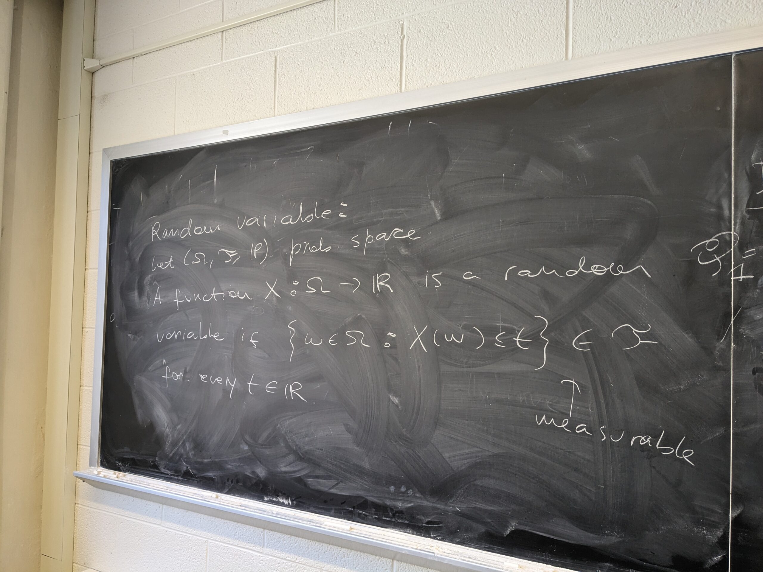
– Definition of probability space (Sample space, sigma-algebra and probability measure)
– Proposition 9.8, page 171: Elementary properties
– Modification of Problem 9.3, page 170: what is the probability that we obtain exactly 50 heads when we throw 100 coins?
– Monty-hall problem. See this lovely video in Numberphile.
Lecture 30
– Problem 9.1, page 170: the Bertrand’s Ballot problem. See page 172 for a solution, or my notes.
Lecture 31
– Definition 9.14, page 175: Conditional Probability
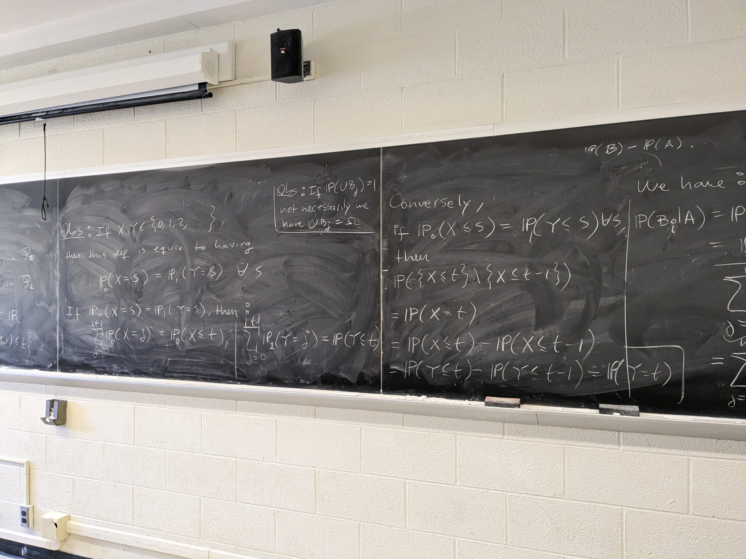
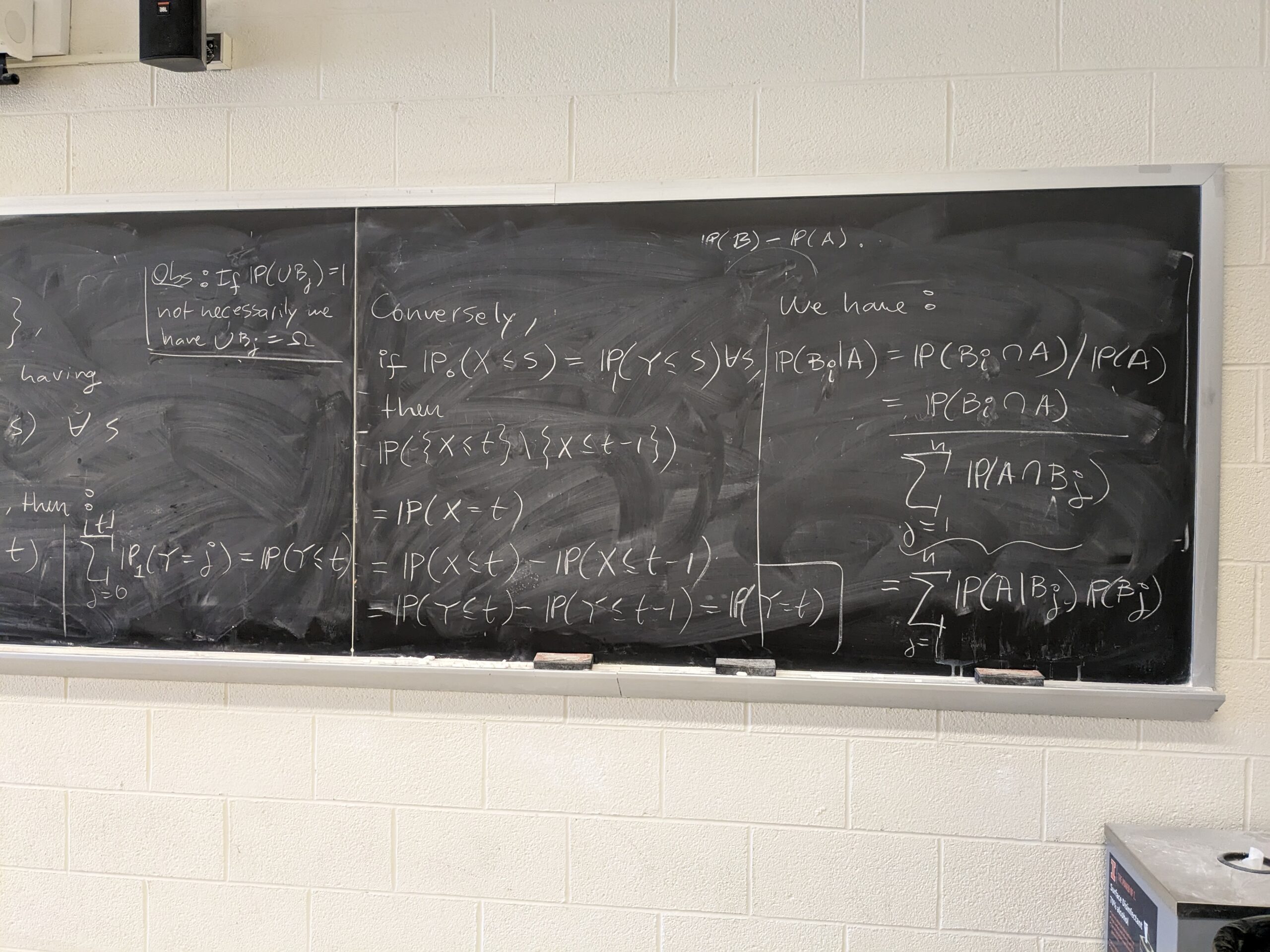
– Proposition 9.18, page 176? Bayes’ Formula
– Conditional probability is a probability measure. See here.
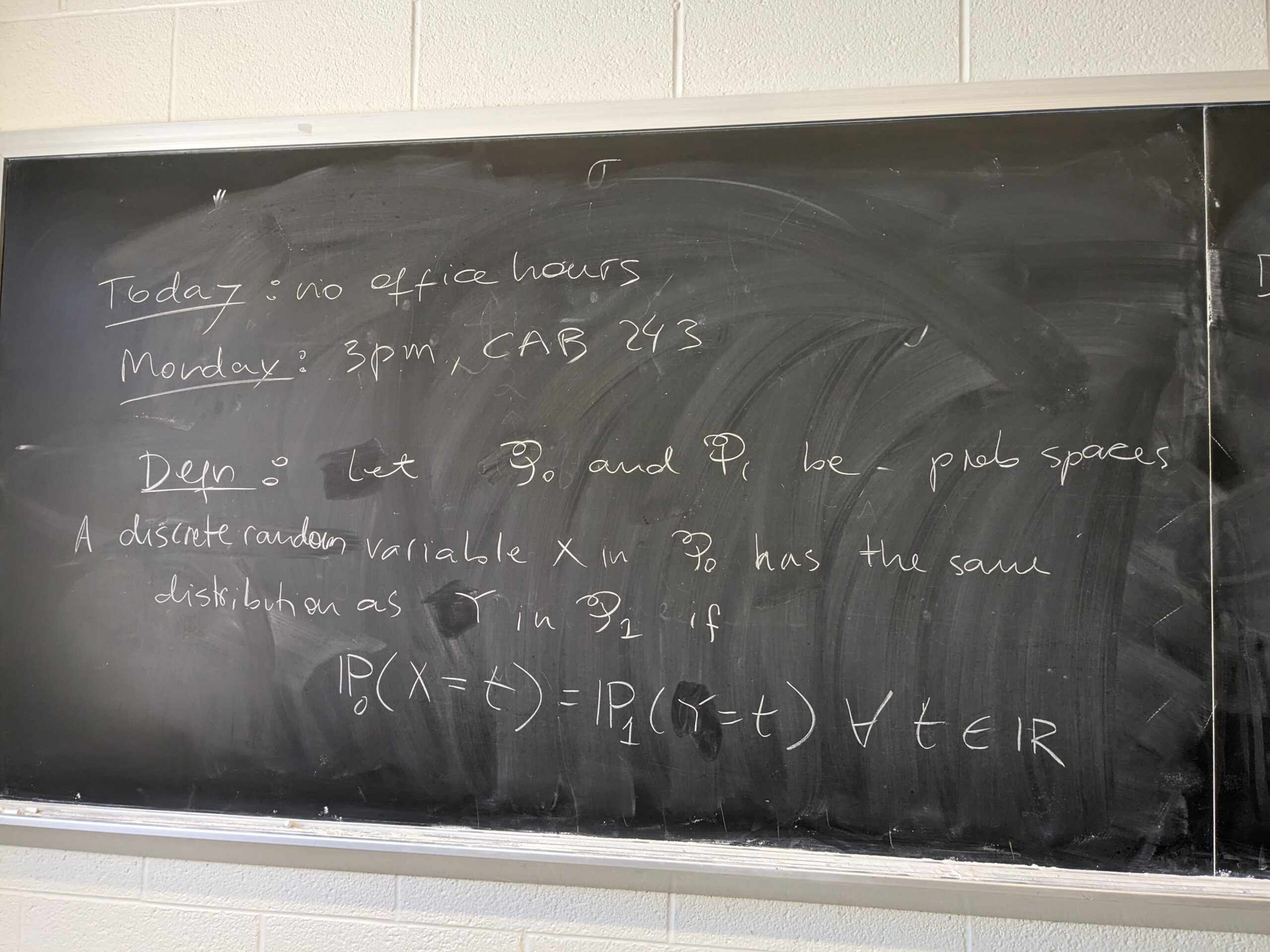
– Identically distributed random variables. See board pictures: 1, 2, 3 and 4.
Lecture 32
– Random variables with the same distribution
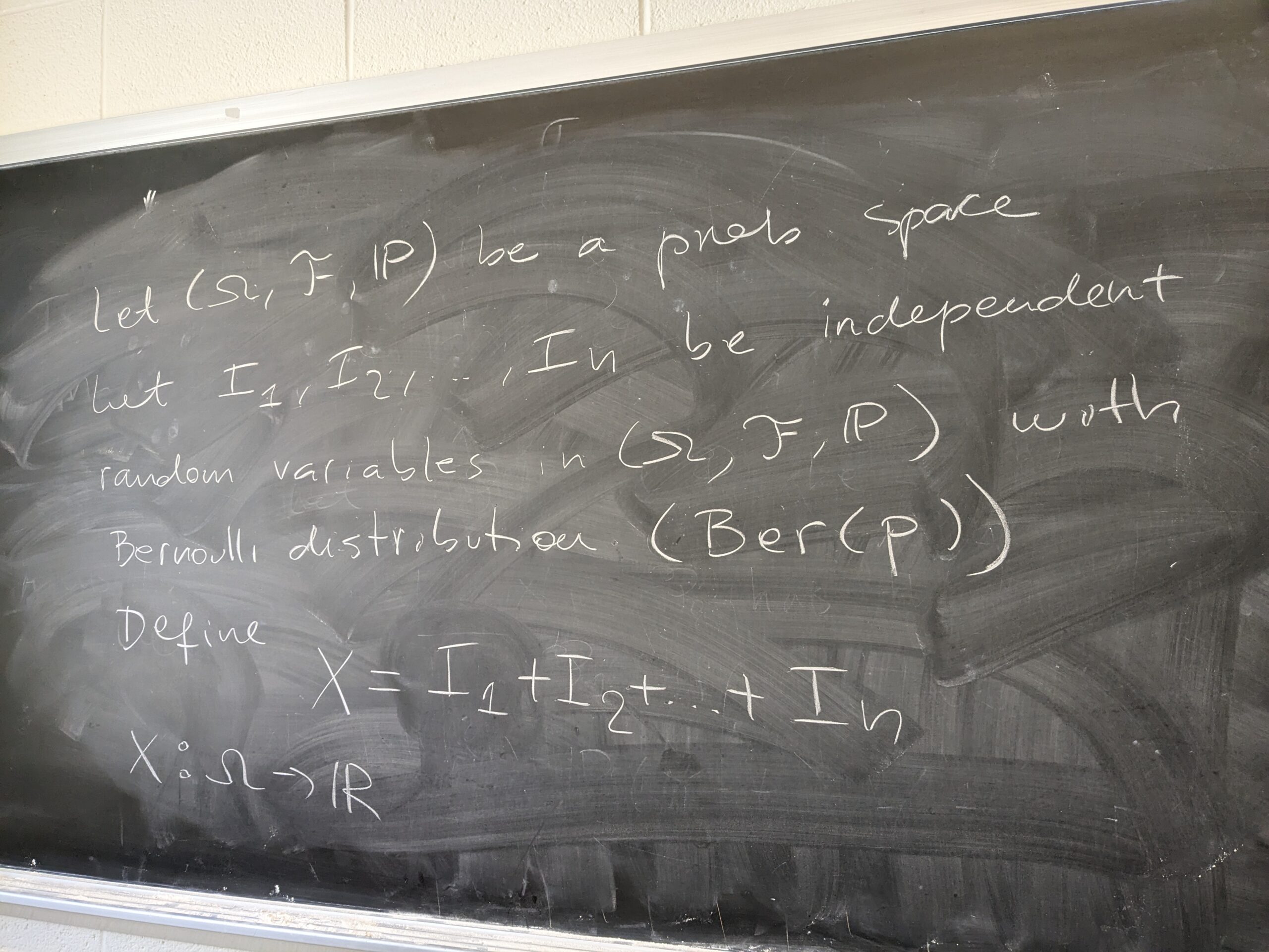
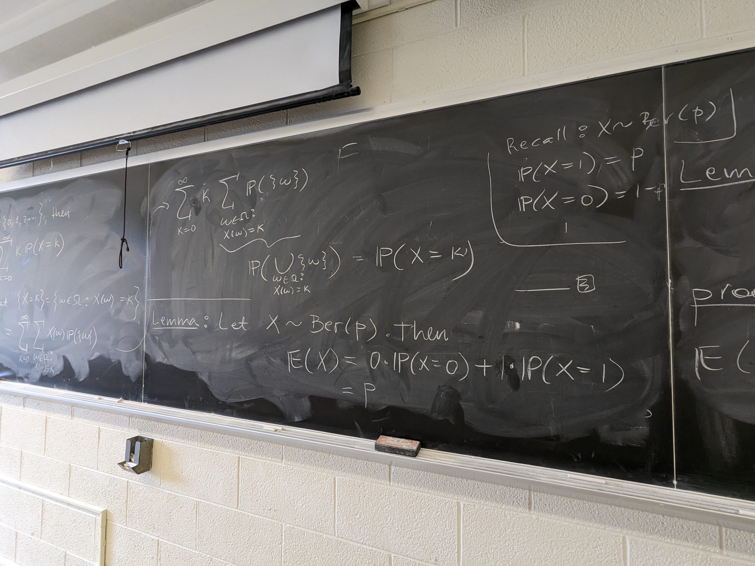
– Bernoulli random variables
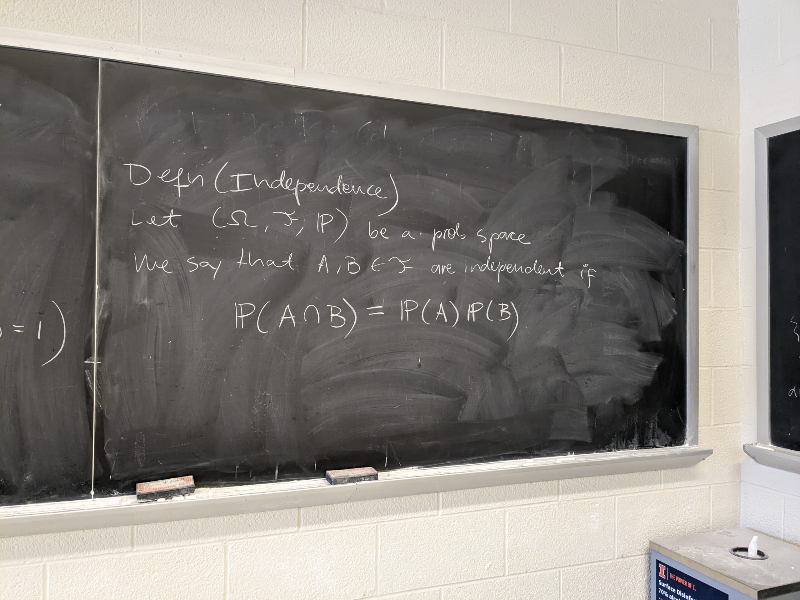
– Independent events
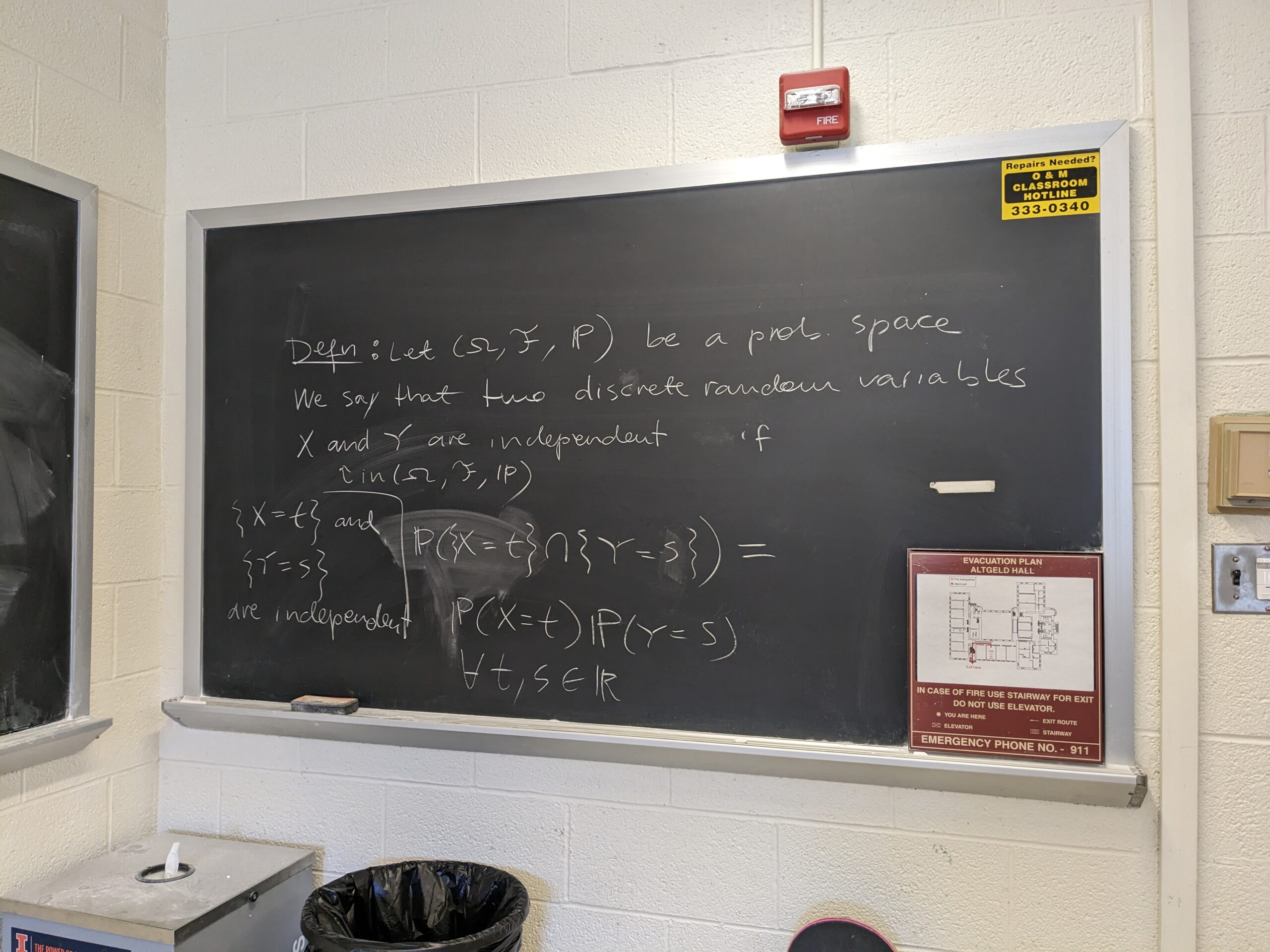
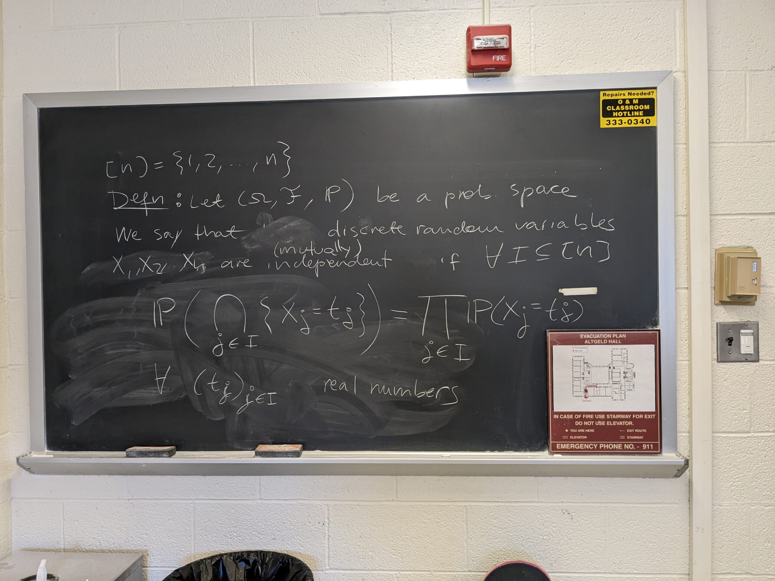
– Independent random variables
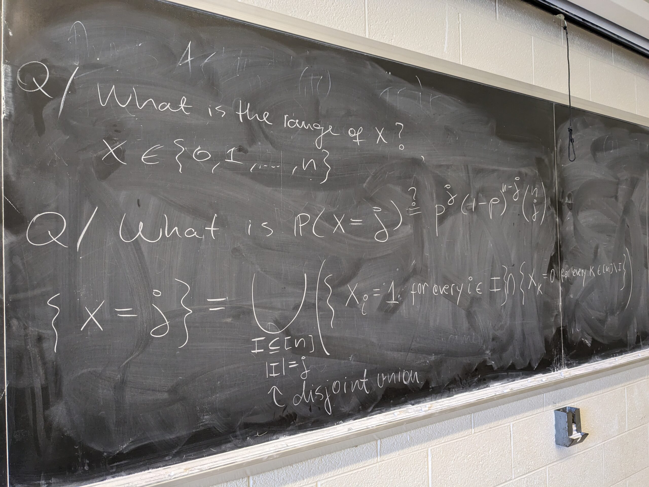
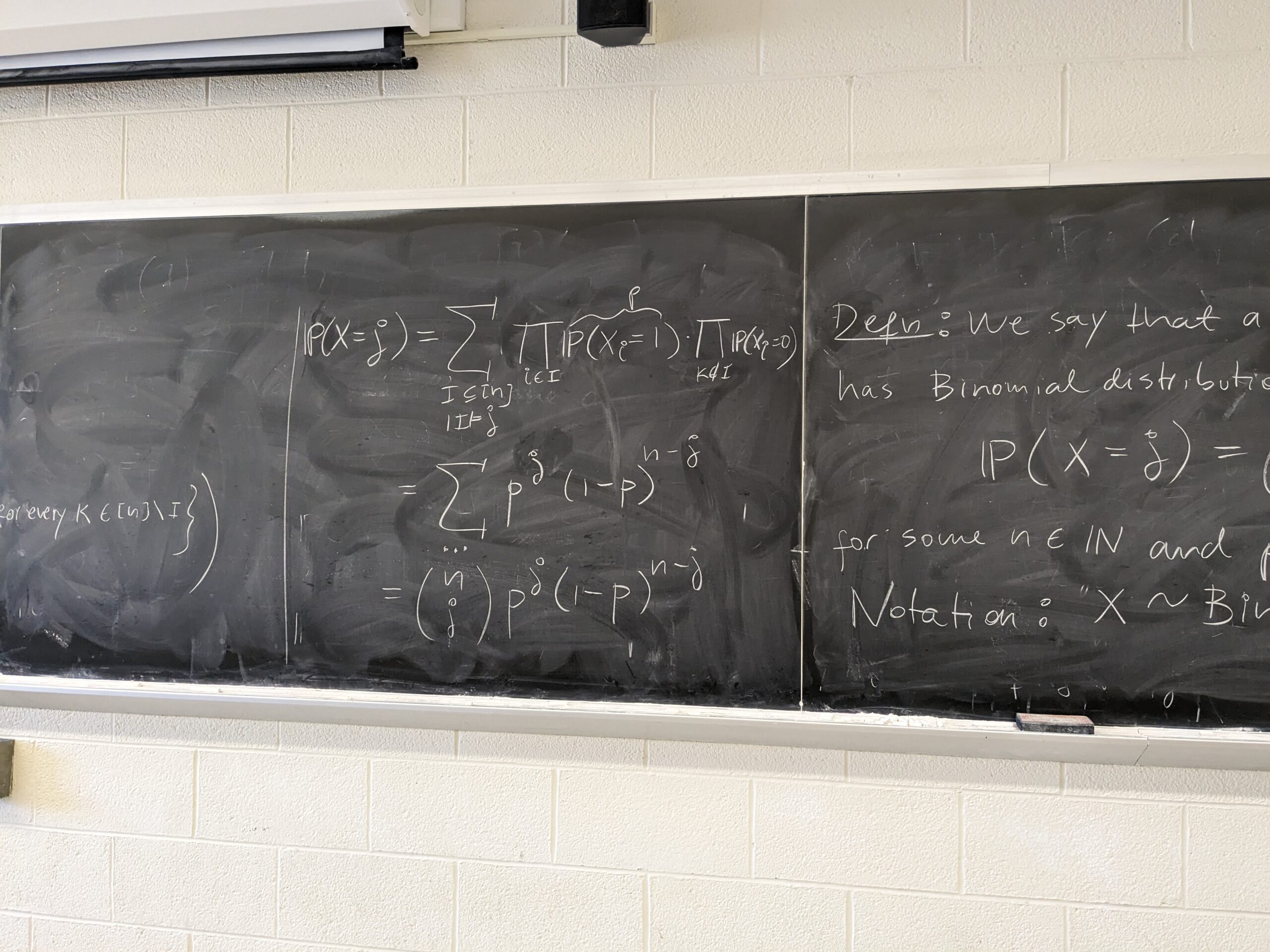
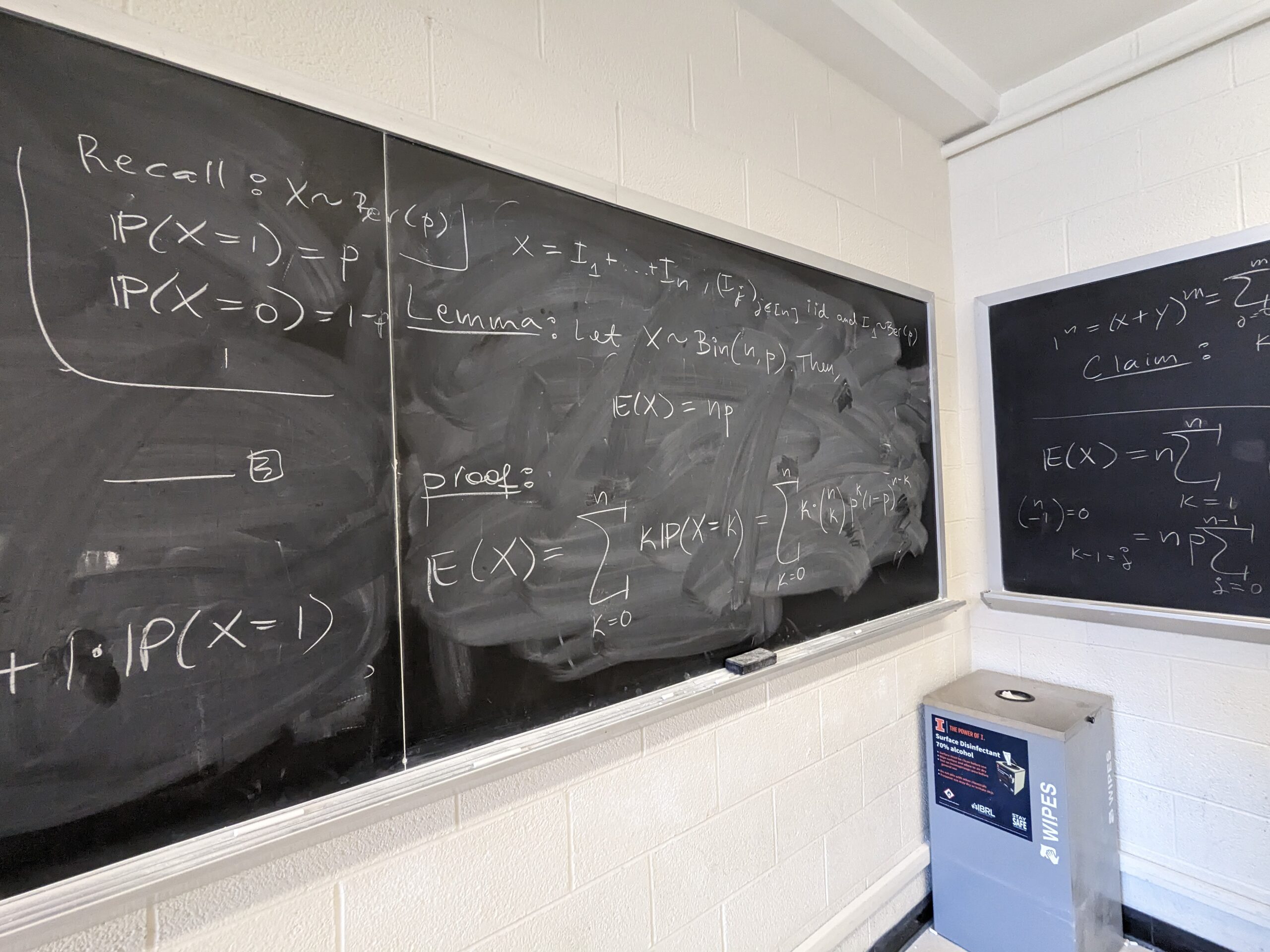
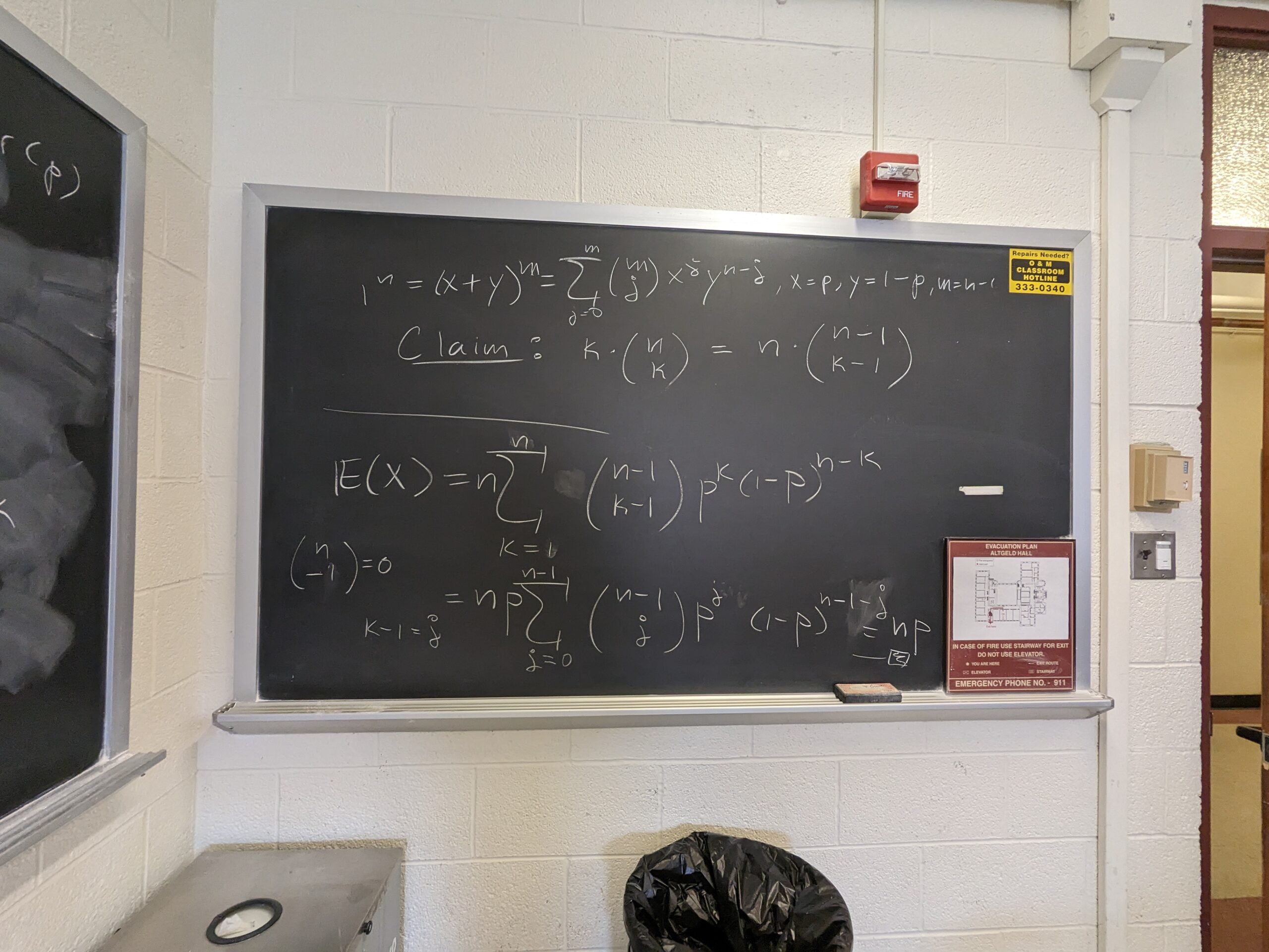
– Binomial distribution
– Geometric distribution
See some of the board pictures here: 1, 2, 3, 4, 5, 6, 7, 8, 9 and 10
Lecture 33
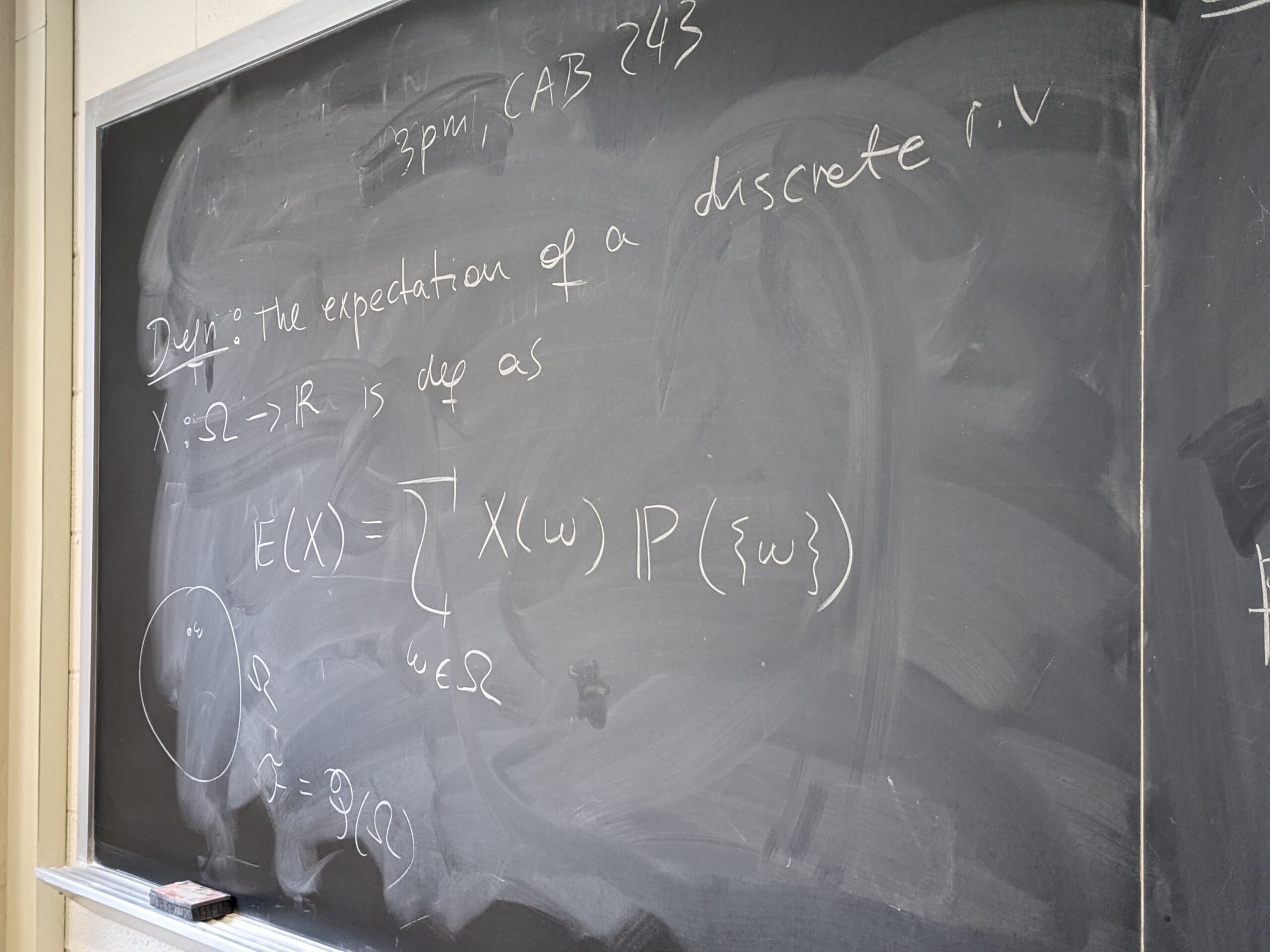
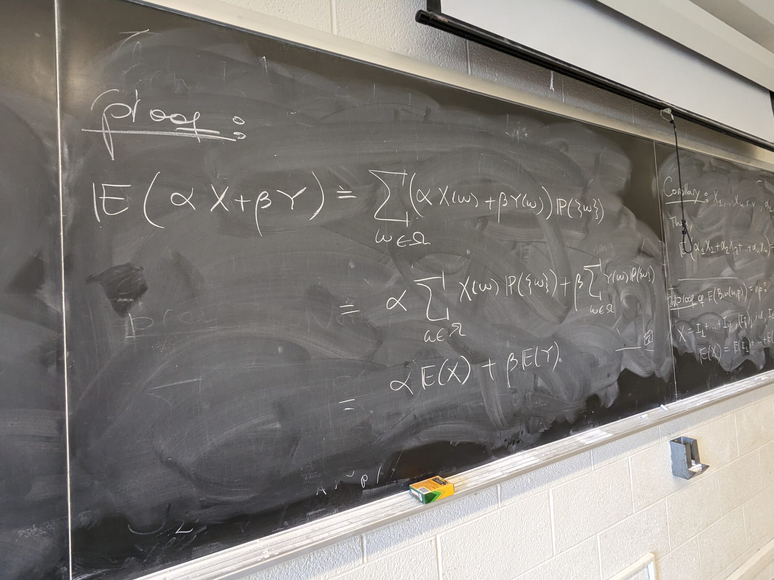
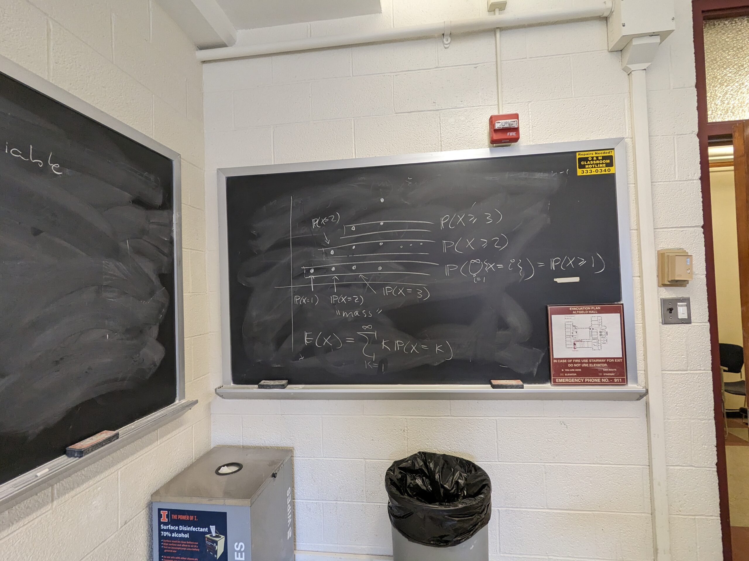
– Definition of expected value
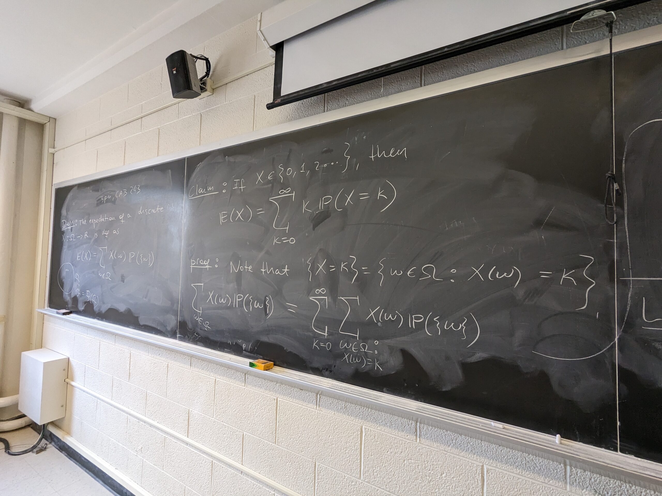
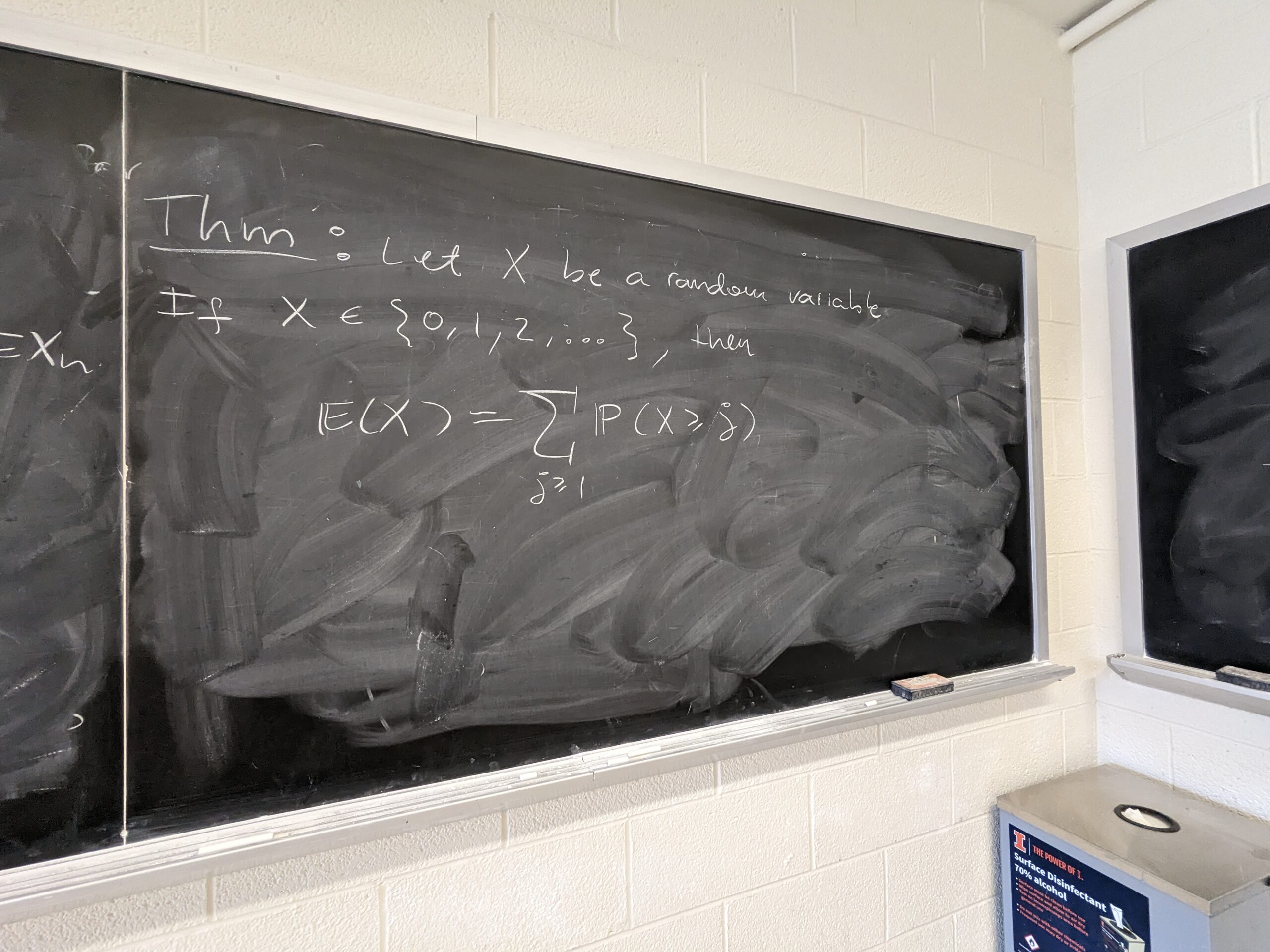
– Expected value of non-negative random variables
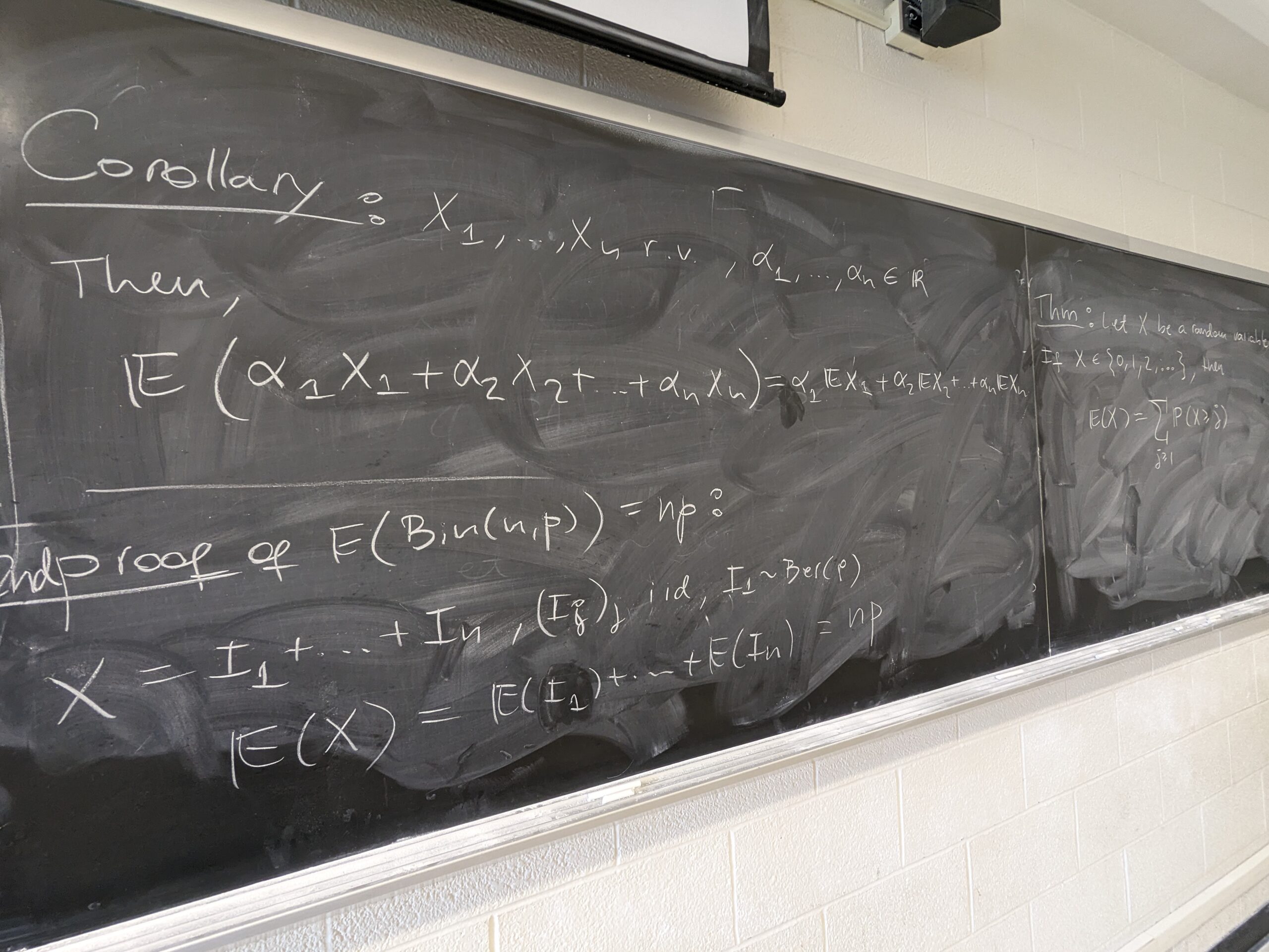
– Expected value of Bernoulli and Binomial random variables
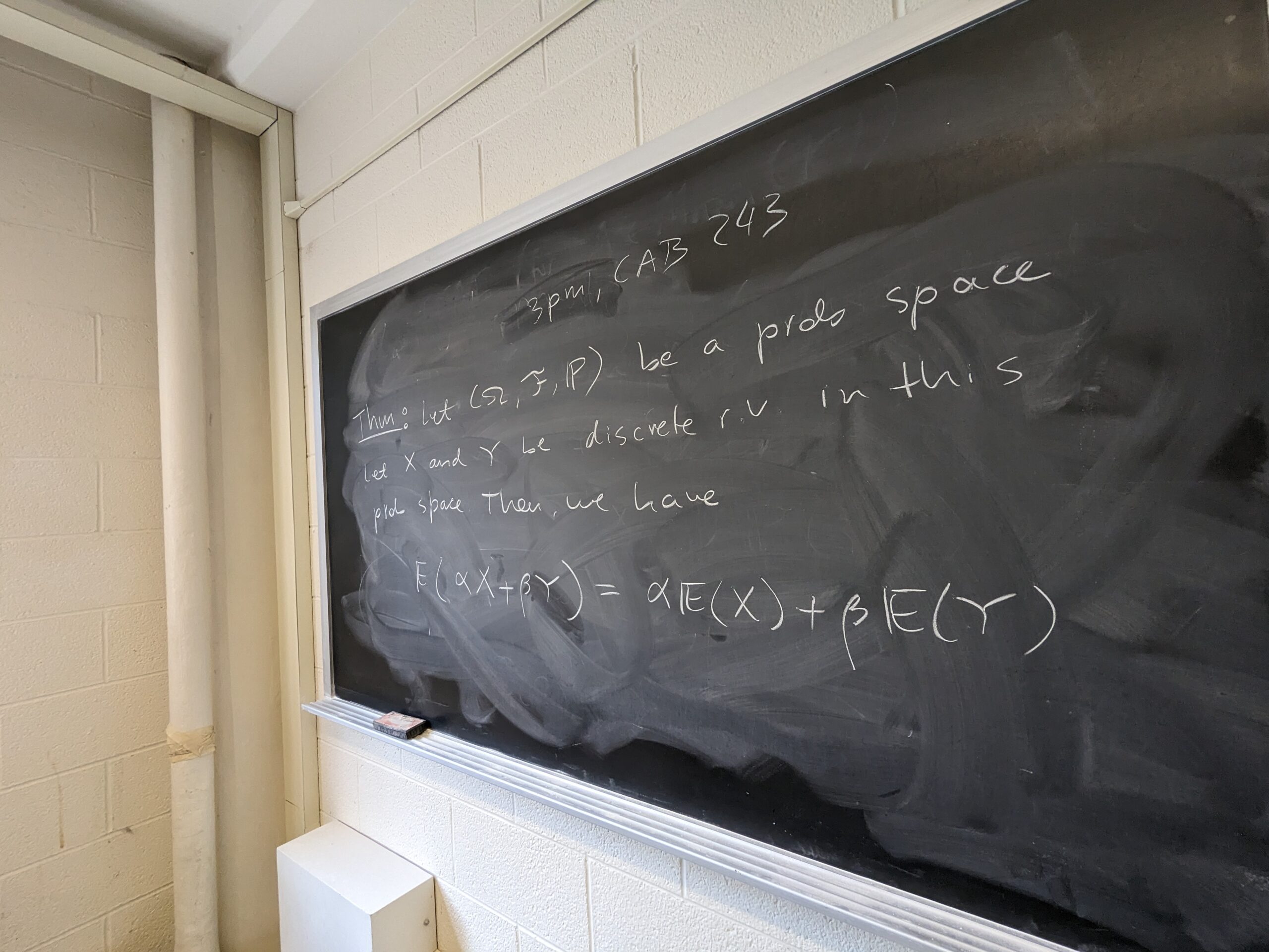
– Linearity of the expectation
– The tail-sum formula
– Expected value of geometric random variables (using the tail-sum formula).
See some of the board pictures here: 1, 2, 3, 4, 5, 6, 7, 8, 9, 10 and 11
Lecture 34
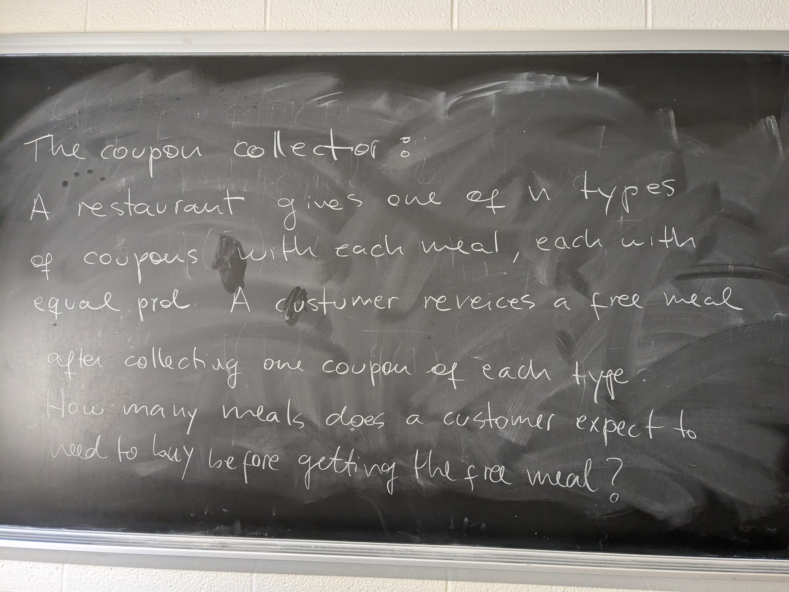
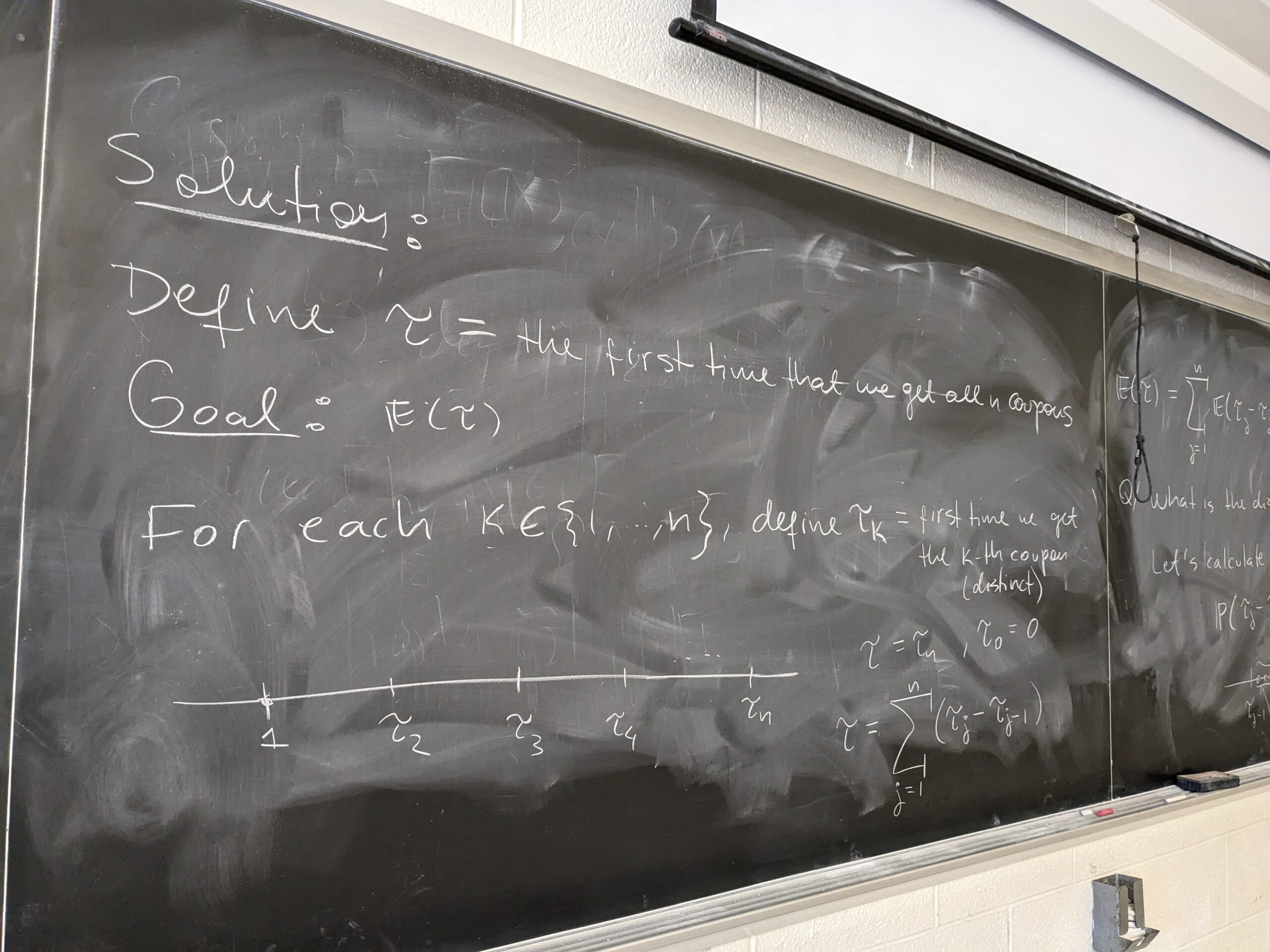
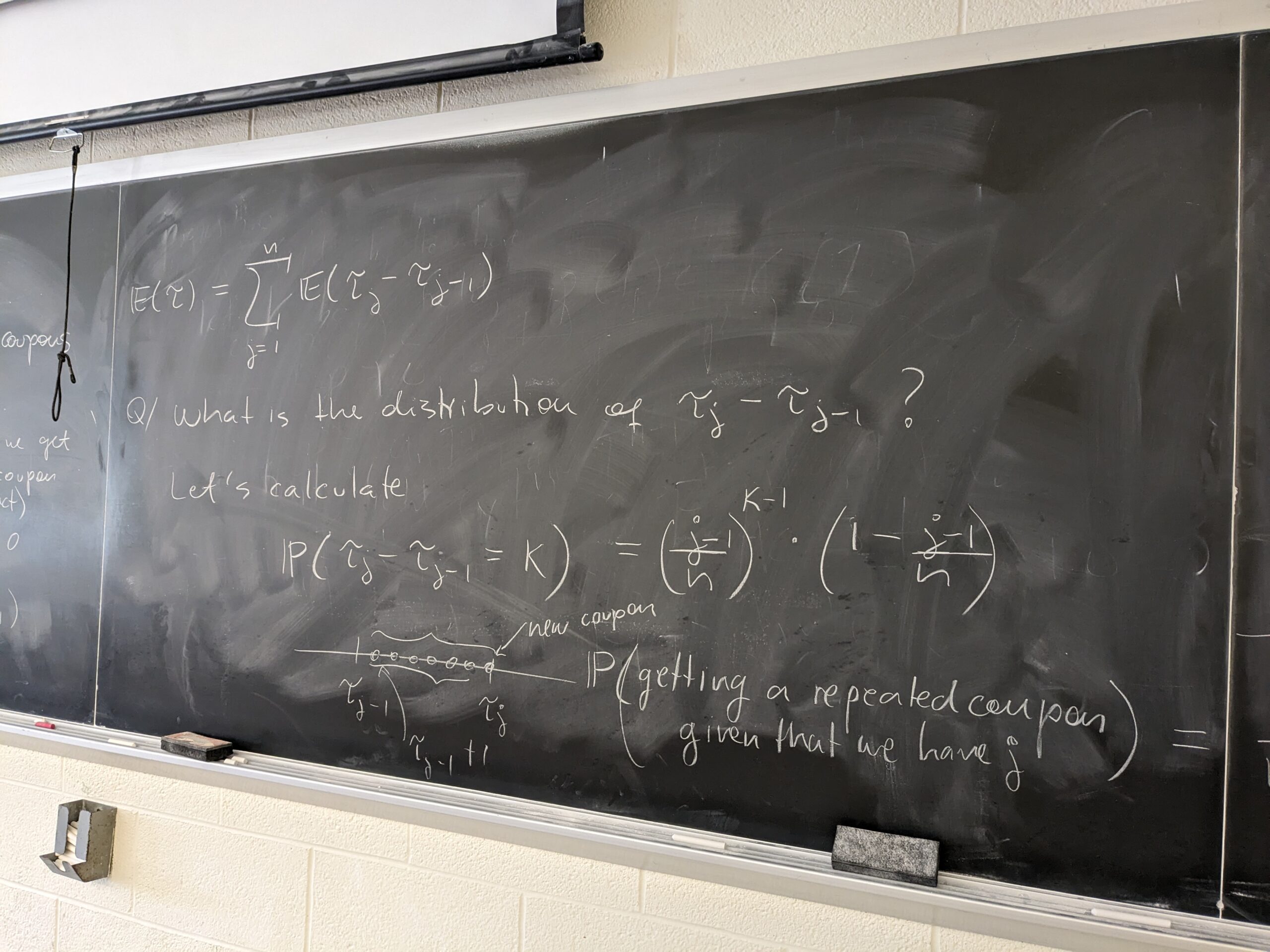
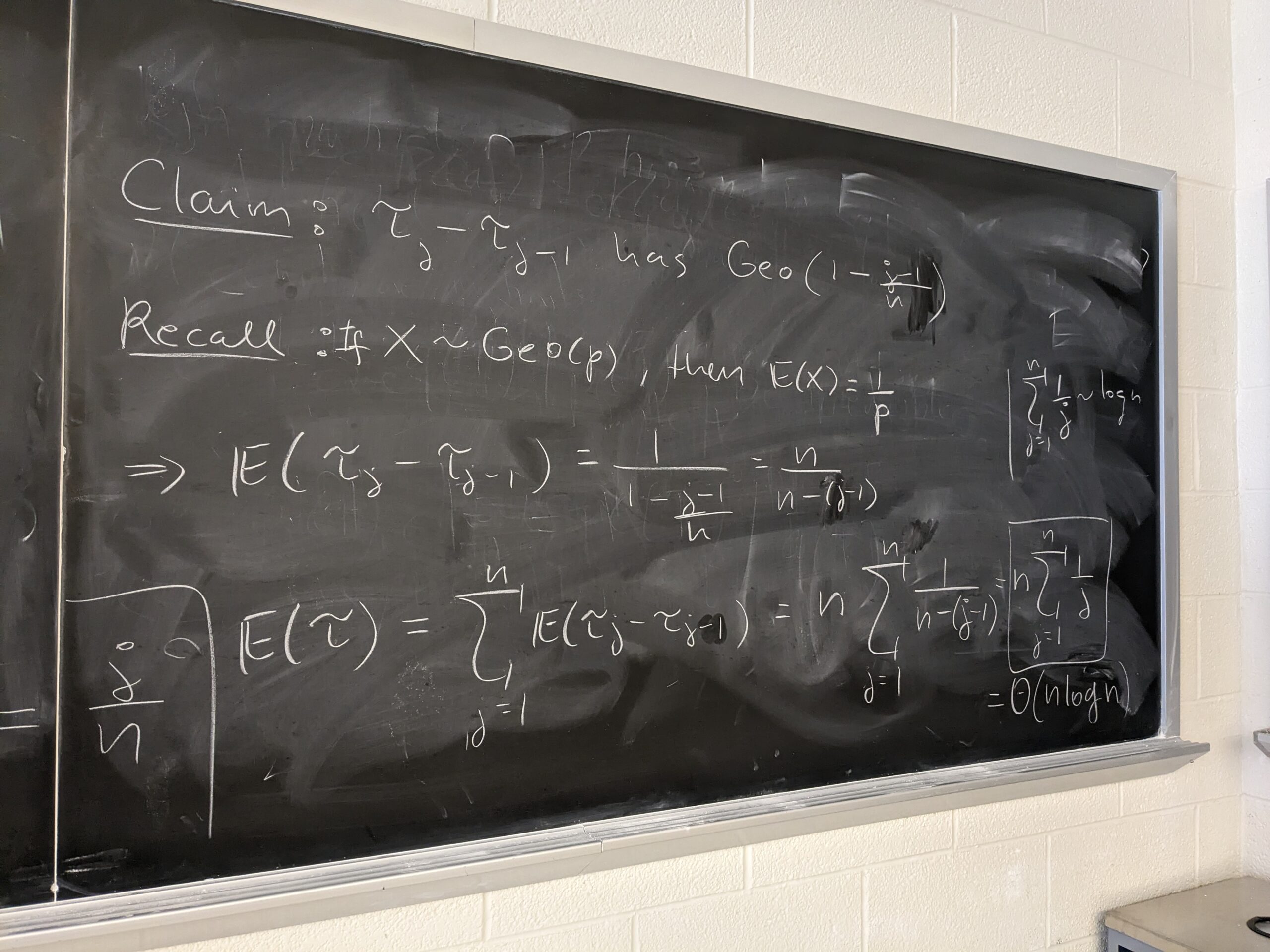
– The coupon collector
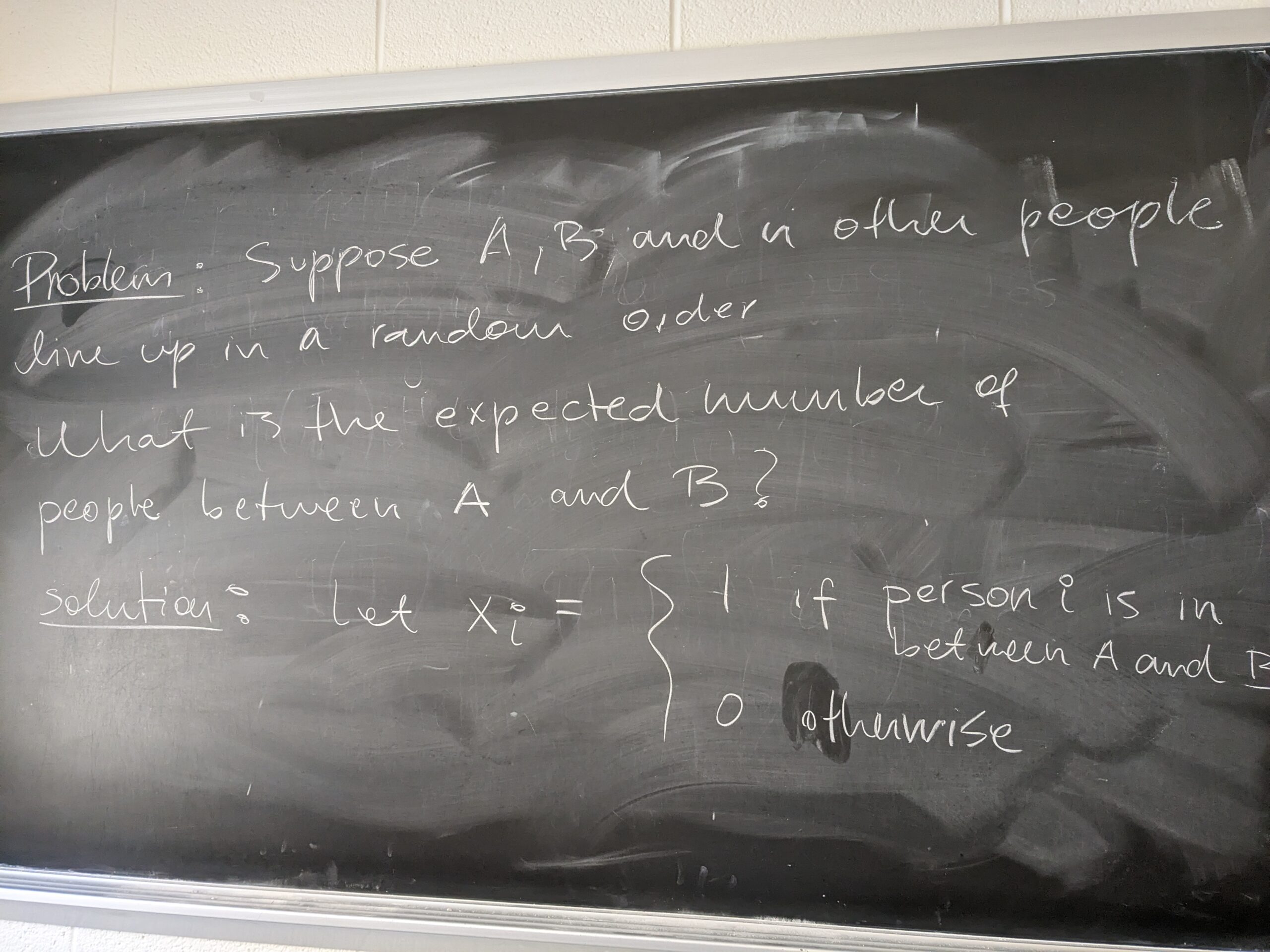
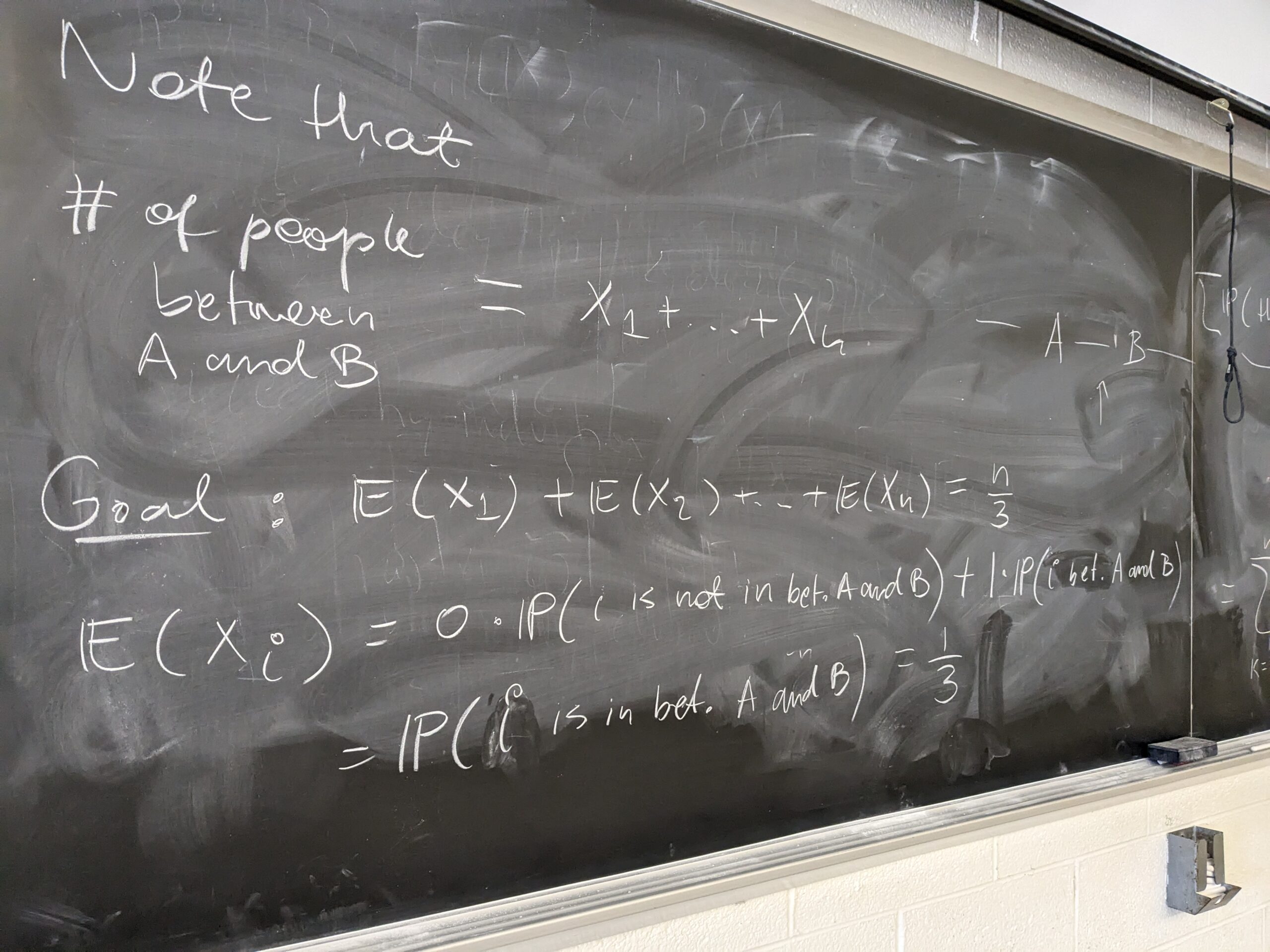
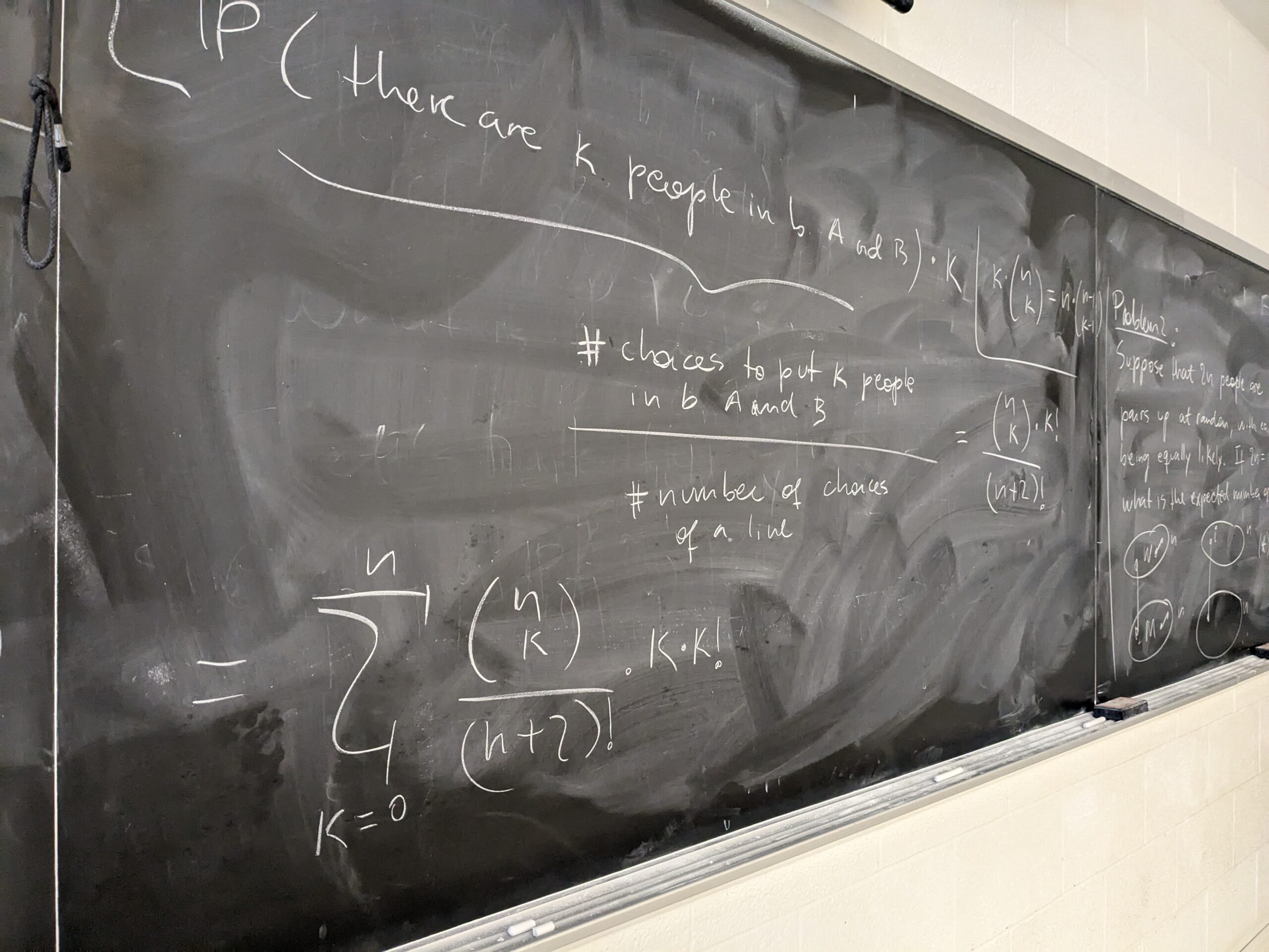
– Problem 1: suppose that A, B and n other people line up in random order. What is the expected number of people between A and B?
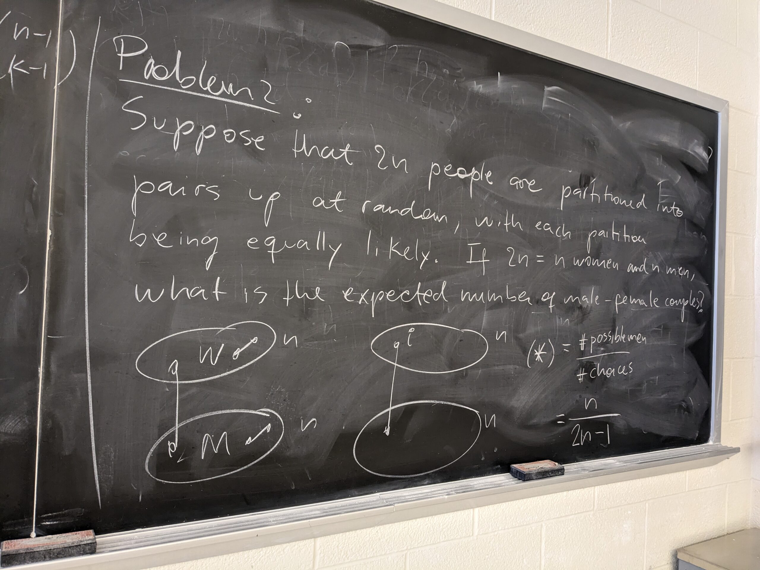
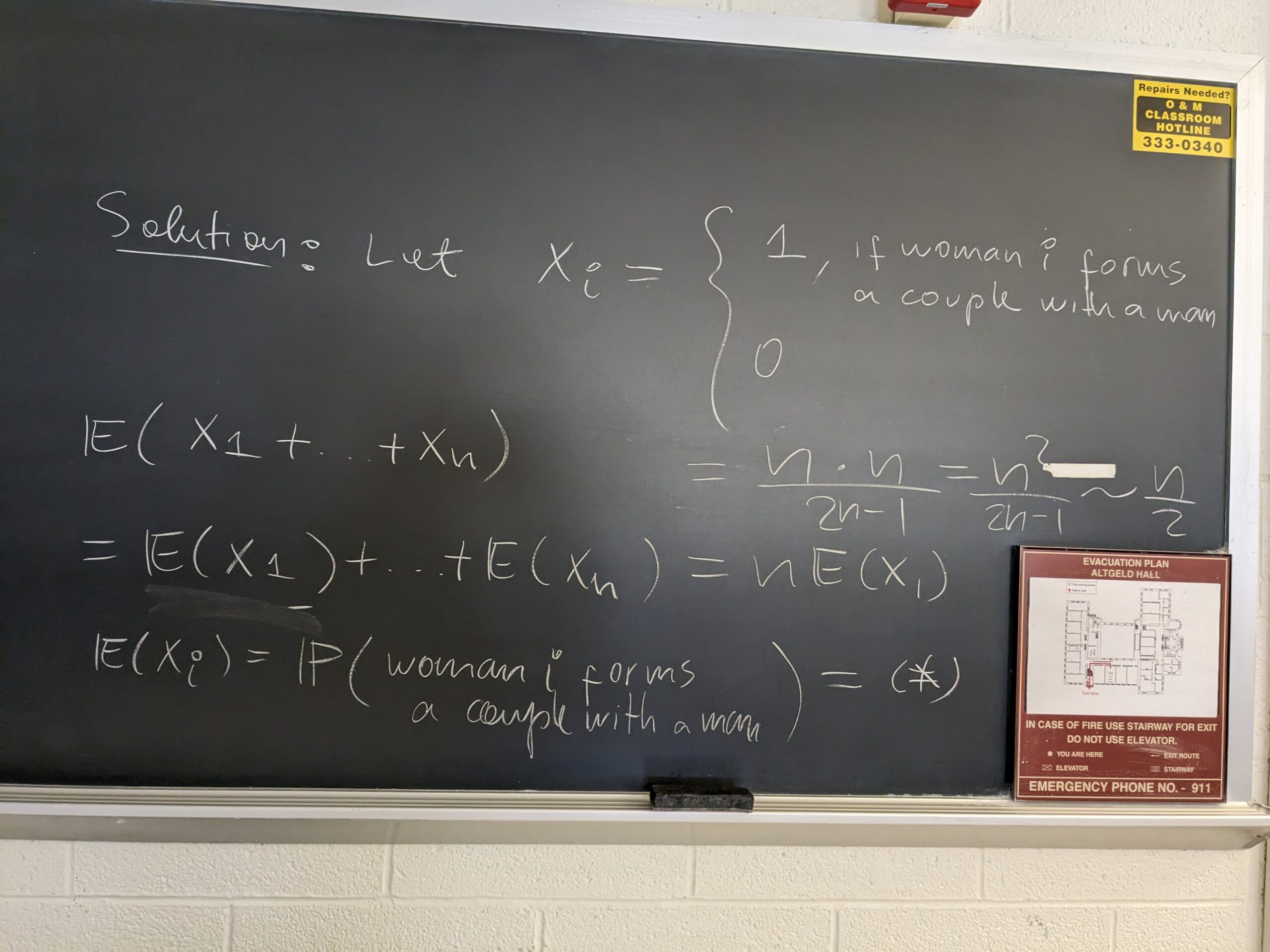
– Problem 2: suppose that 2n people are partitioned into pairs at random, which each partition being equally likely. If there are n men and n women, what is the expected number of male-female coupes?
See some of the board pictures here: 1, 2, 3, 4, 5, 6, 7, 8 and 9
Lecture 35
– We Reviewed the content of the third midterm
Lecture 36
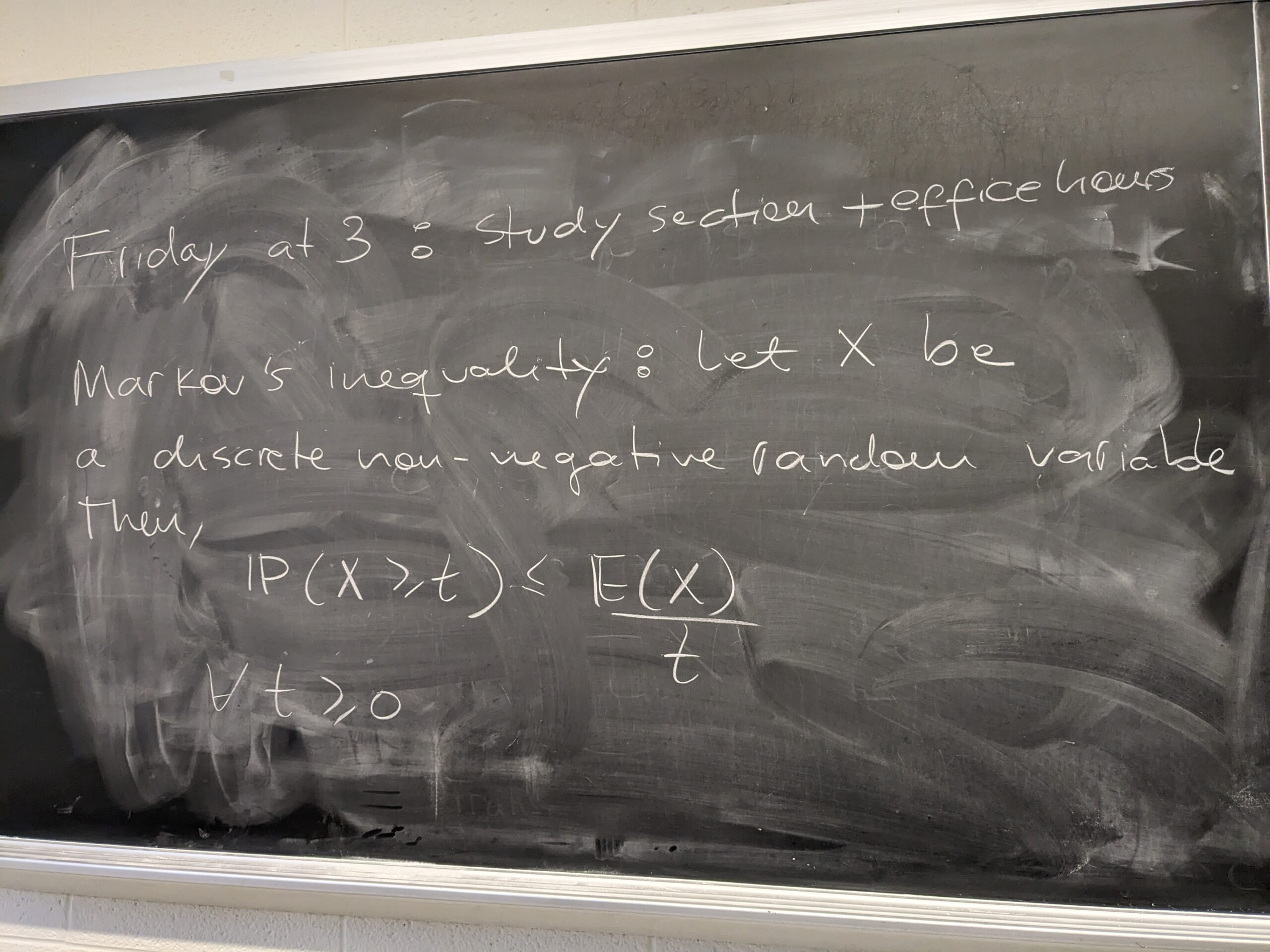
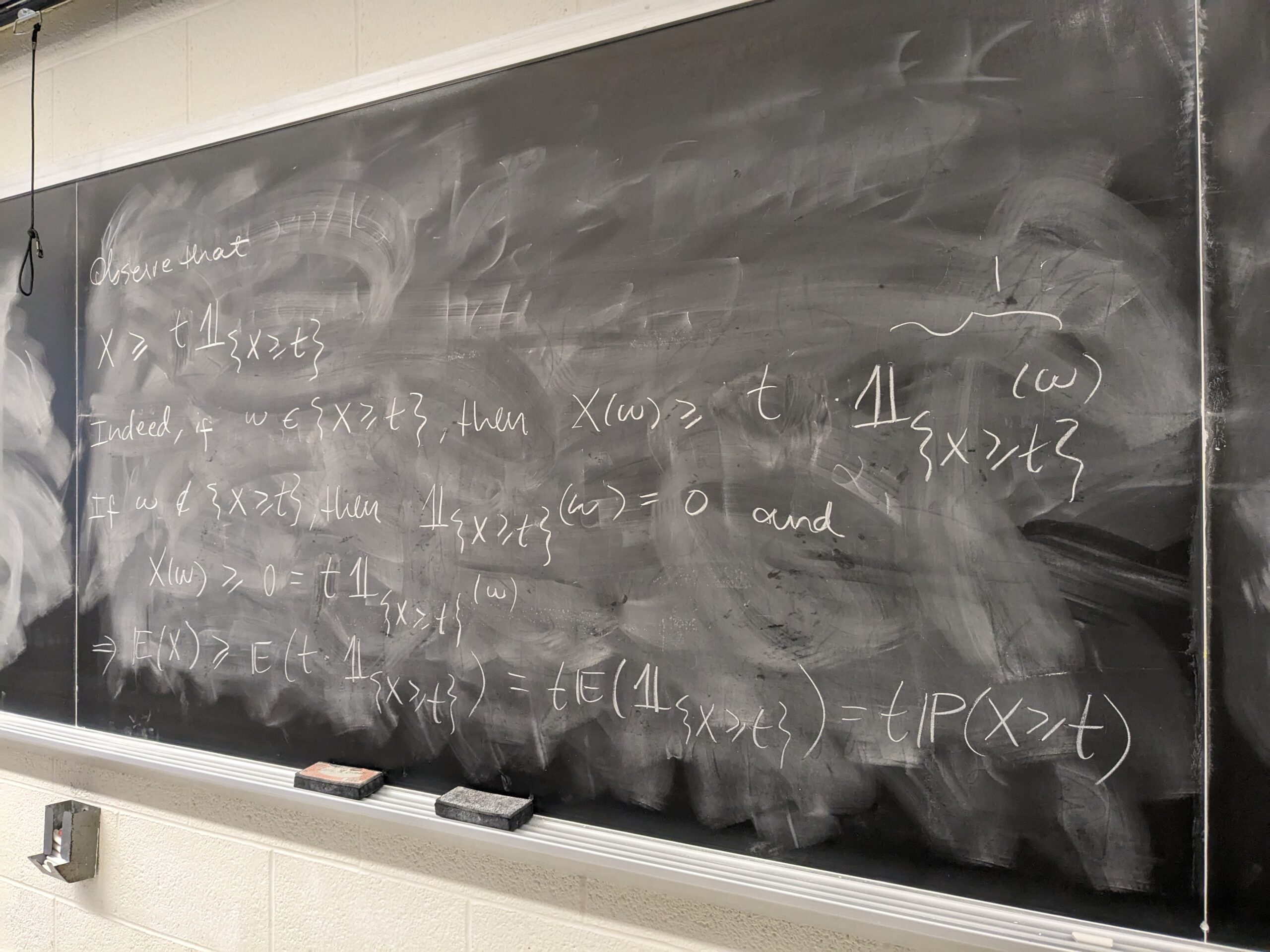
– Markov’s inequality
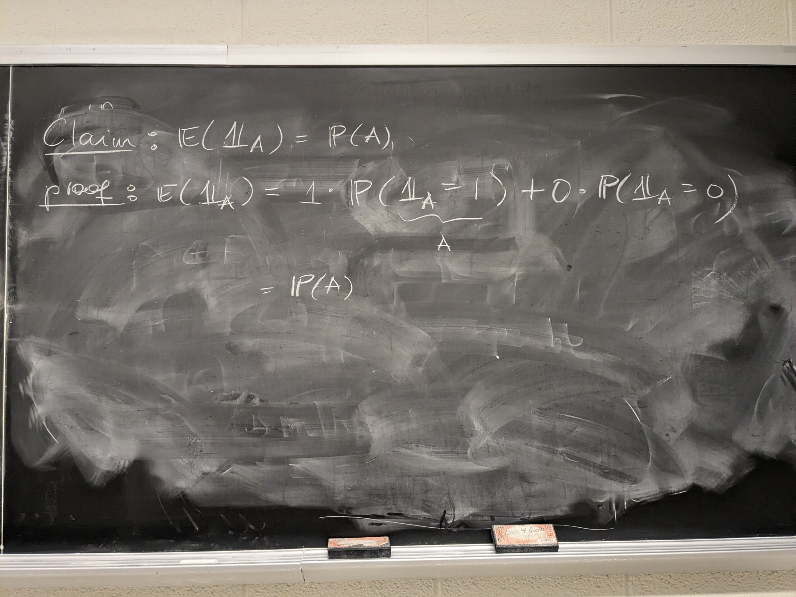
– Indicator functions (definition and expectation)
– Recalling what are independent random variables
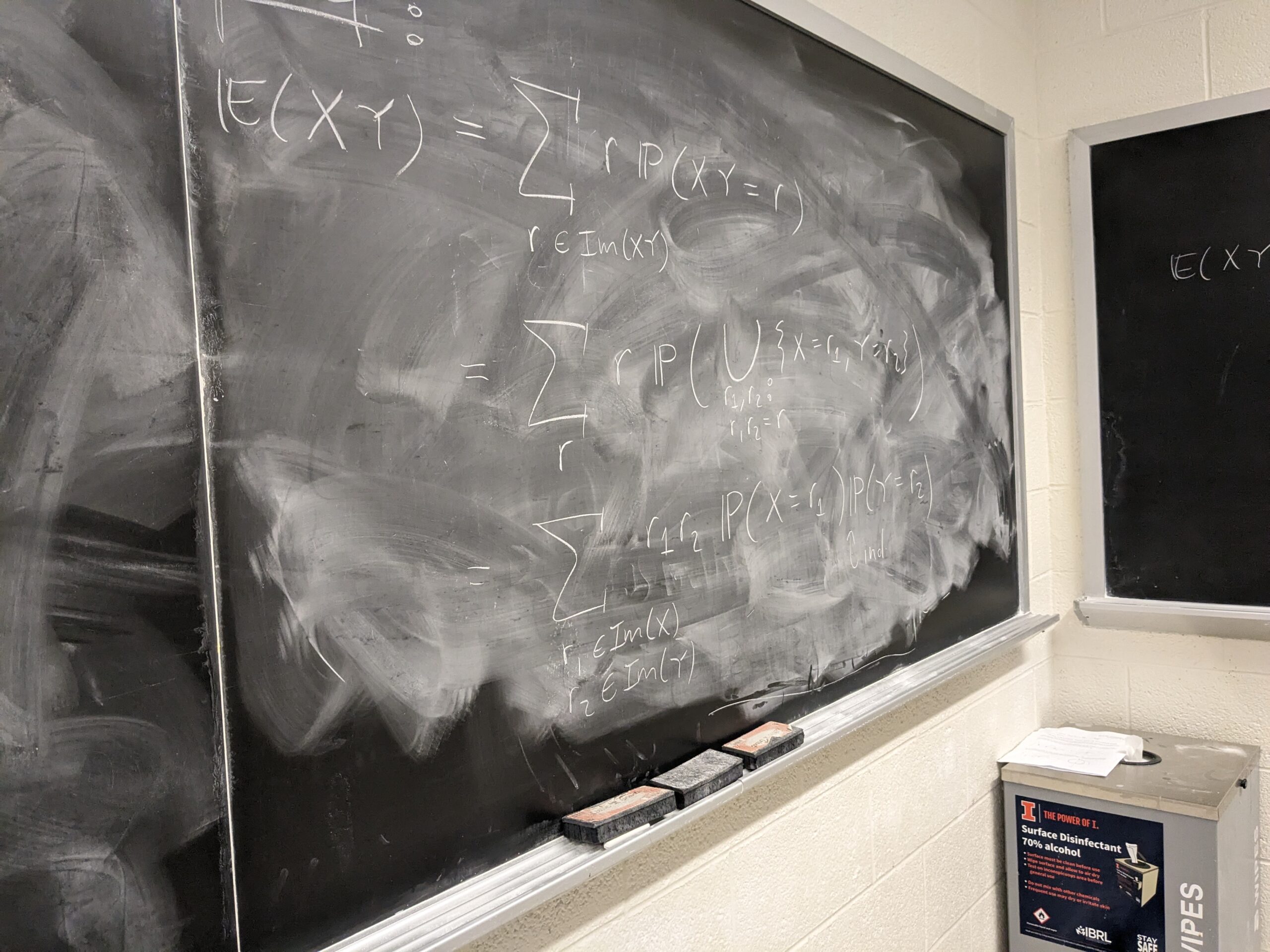
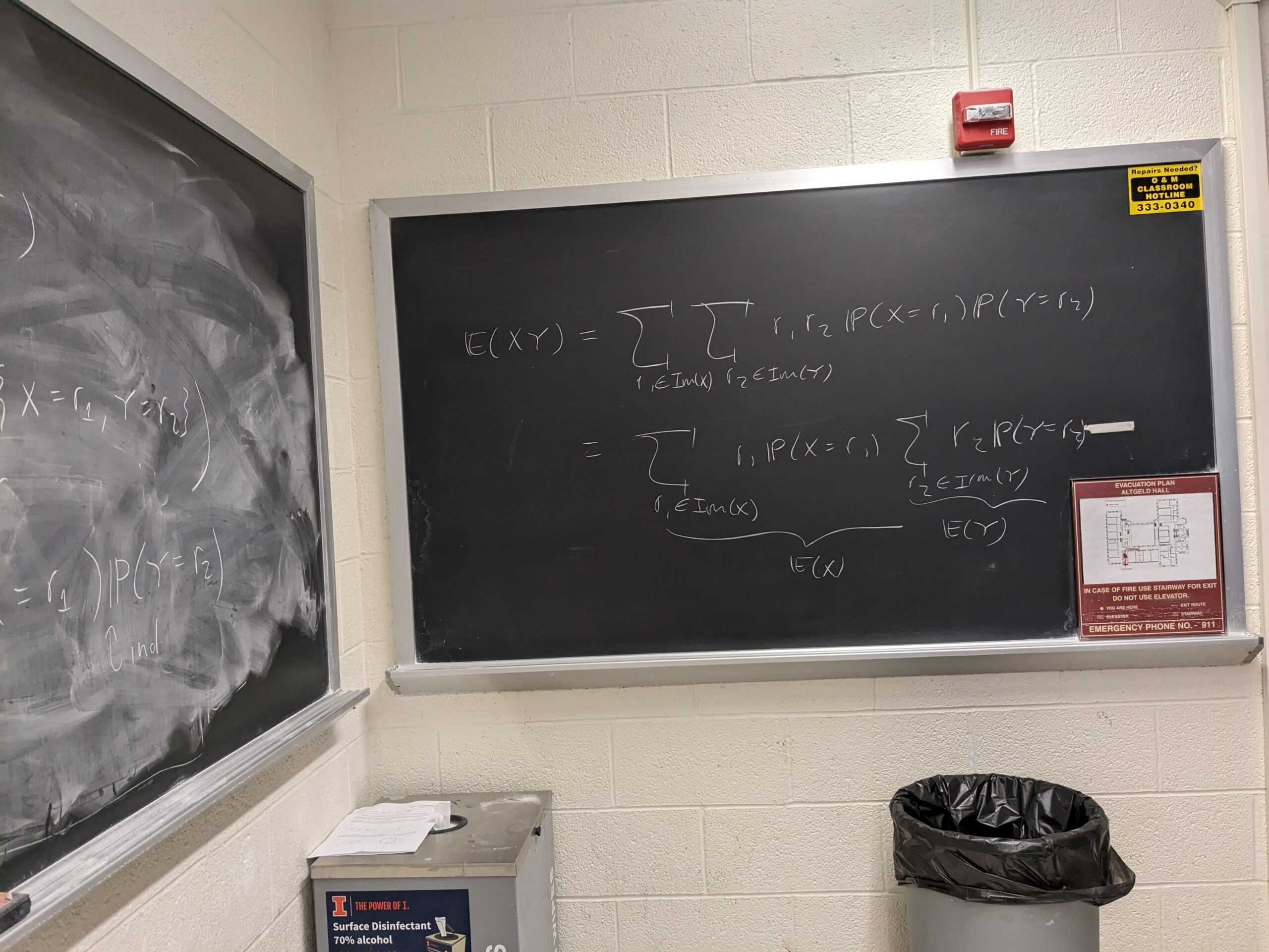
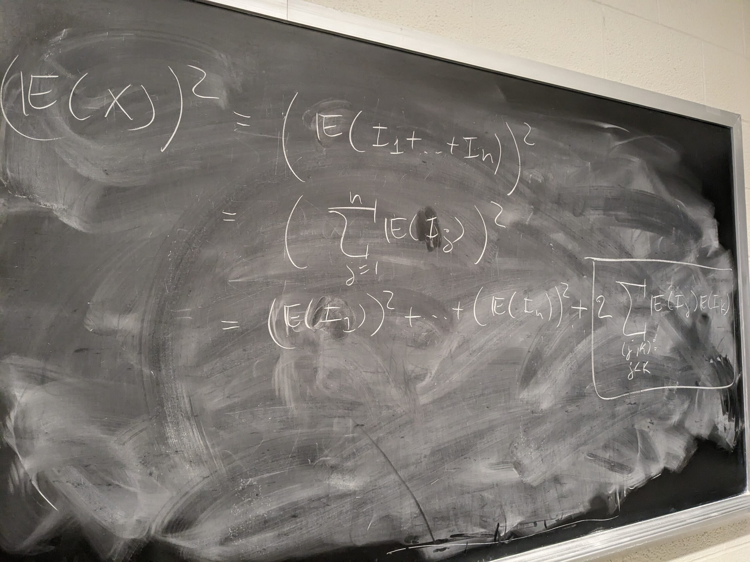
– If X and Y are independent discrete random variables, then \mathbb{E}(XY) = \mathbb{E}(X)\mathbb{E}(Y)
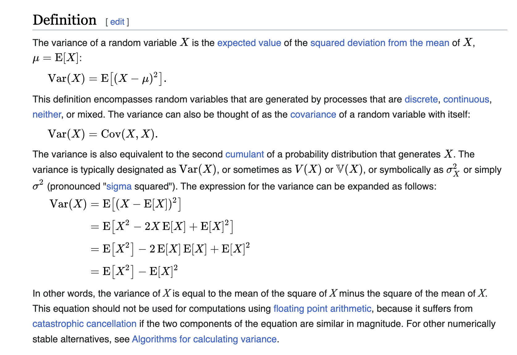
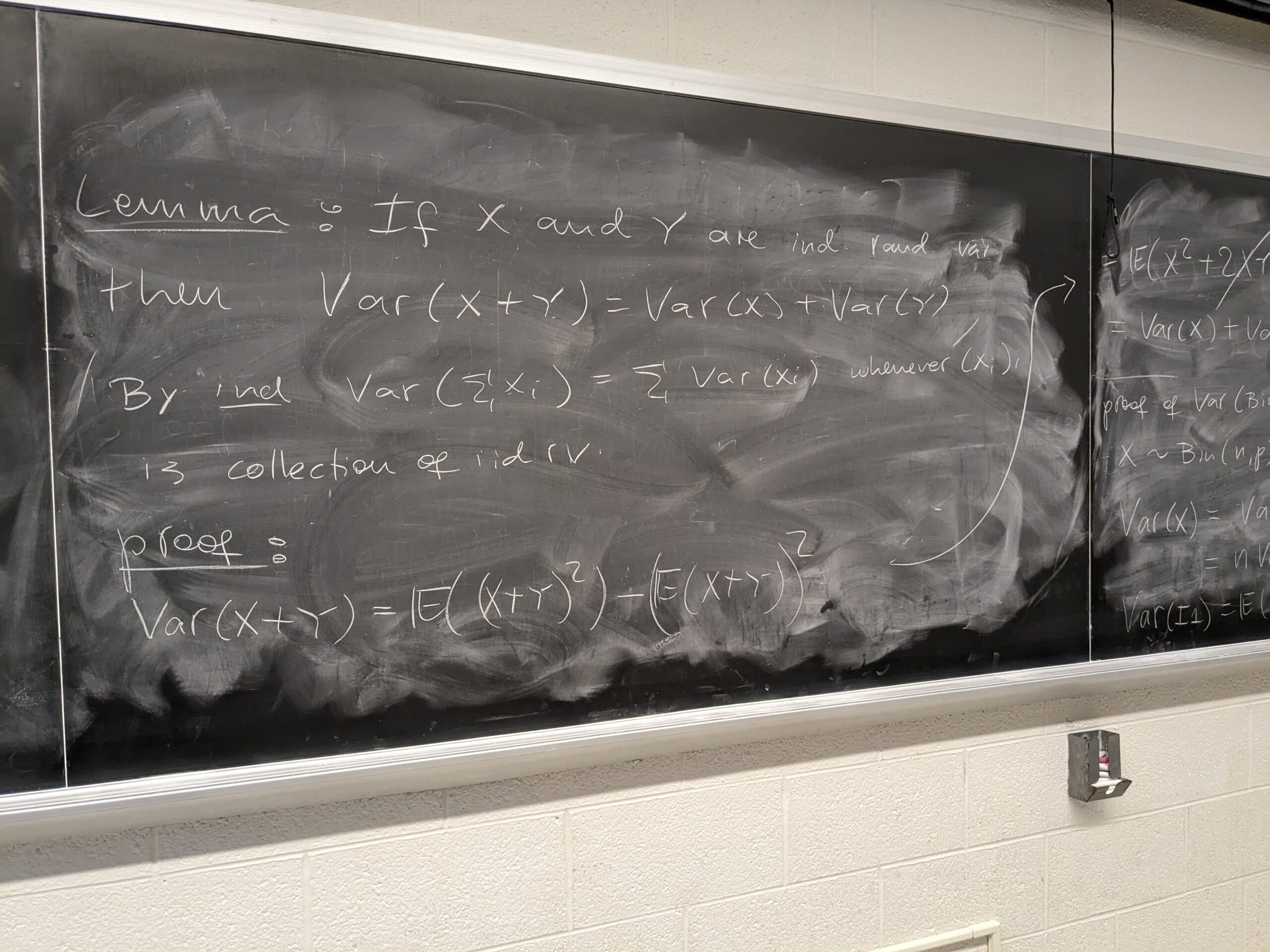
– Definition of Variance
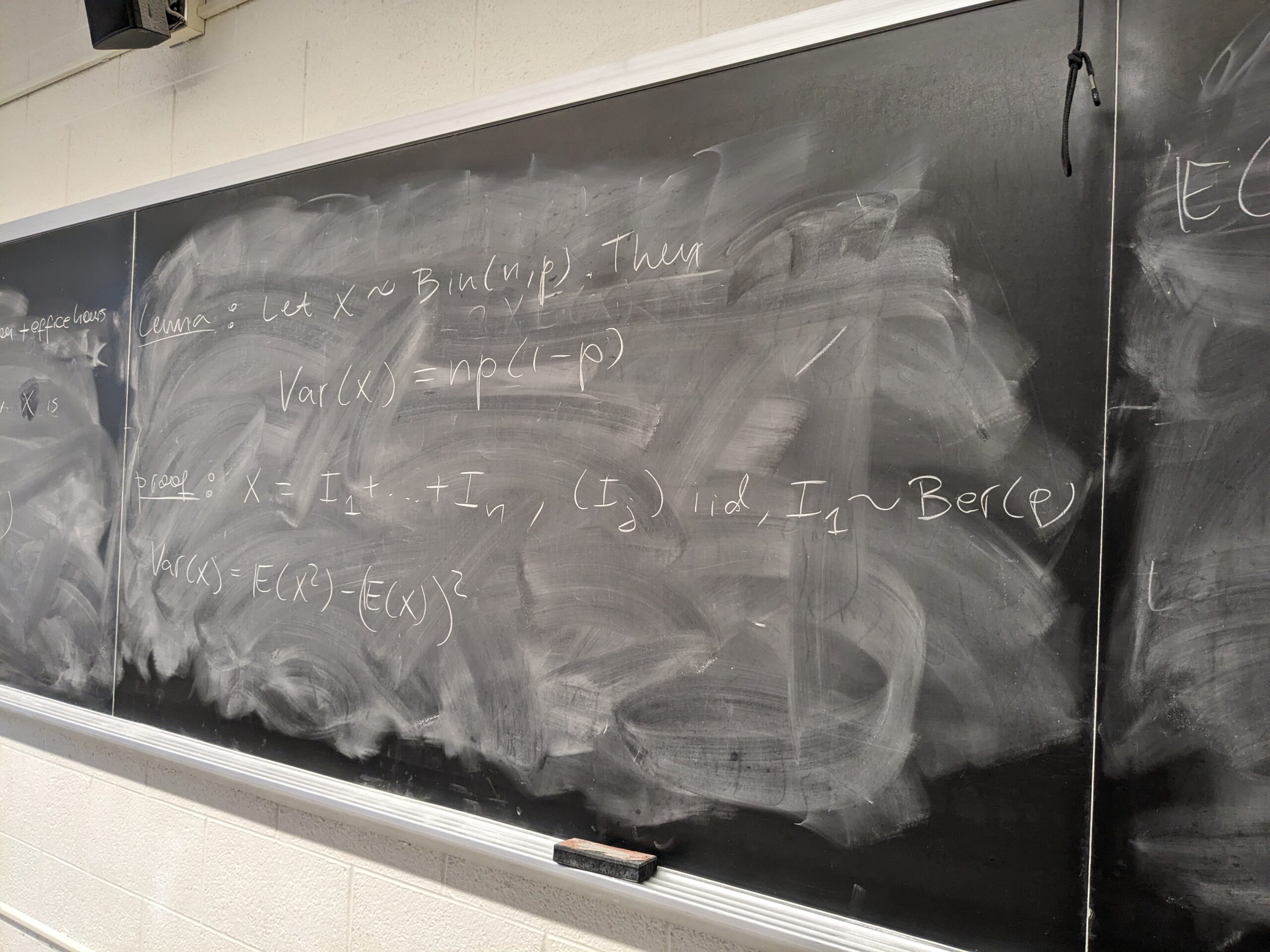
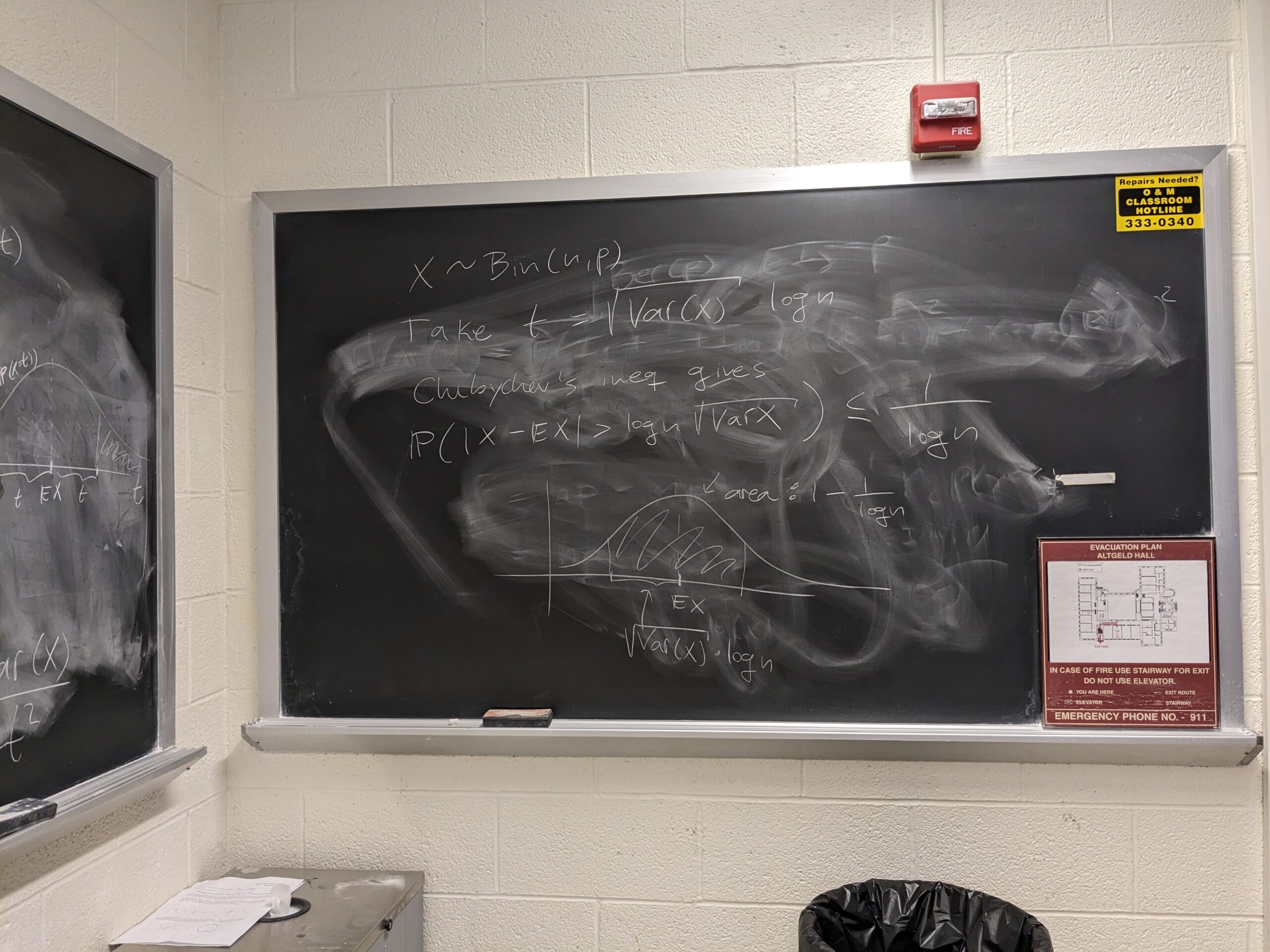
– The variance of a binomial random variable \text{Bin}(n,p) is np(1-p)
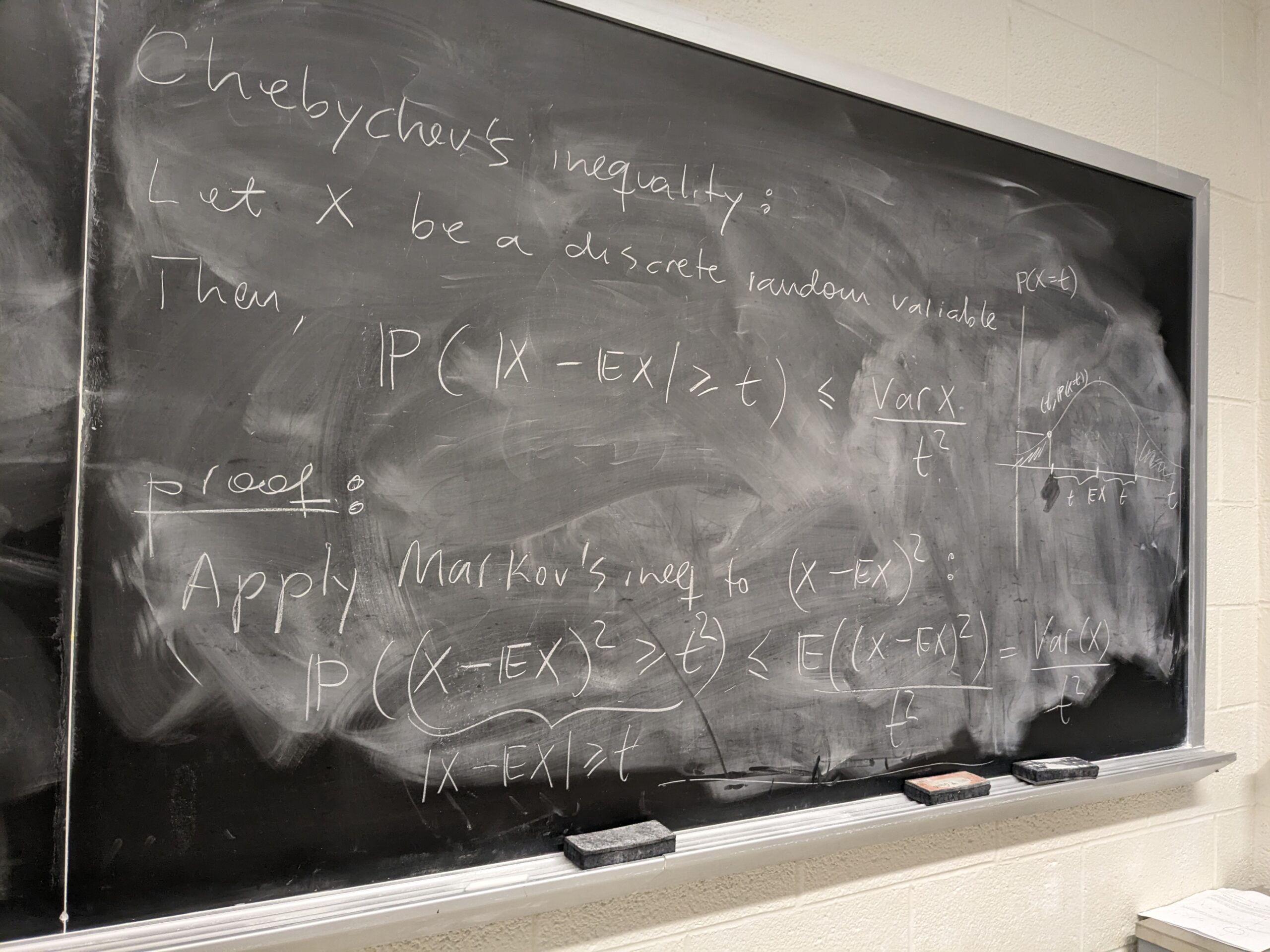
– Chebyshev’s inequality
See some of the board pictures here: 1, 2, 3, 4, 5, 6, 7, 8, 9, 10, 11, 12, 13, 14 and 15.
Lecture 37
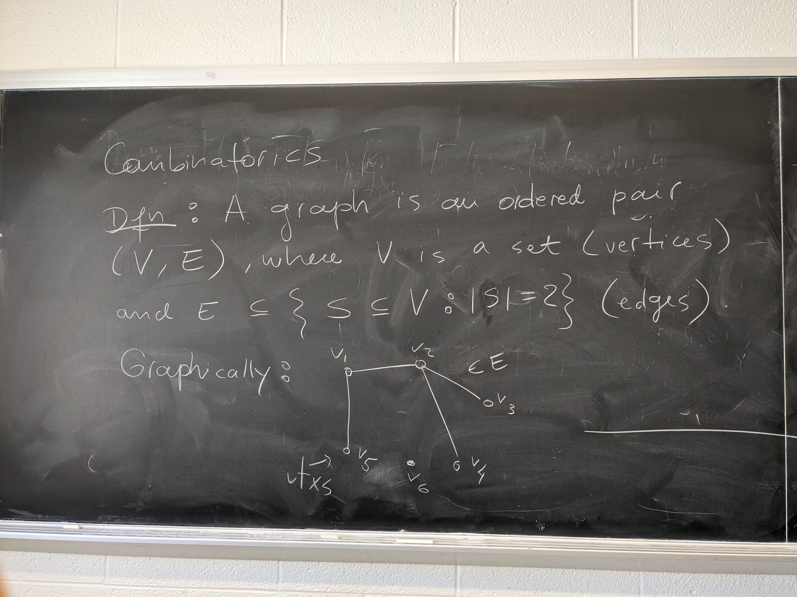
– Definition of graph
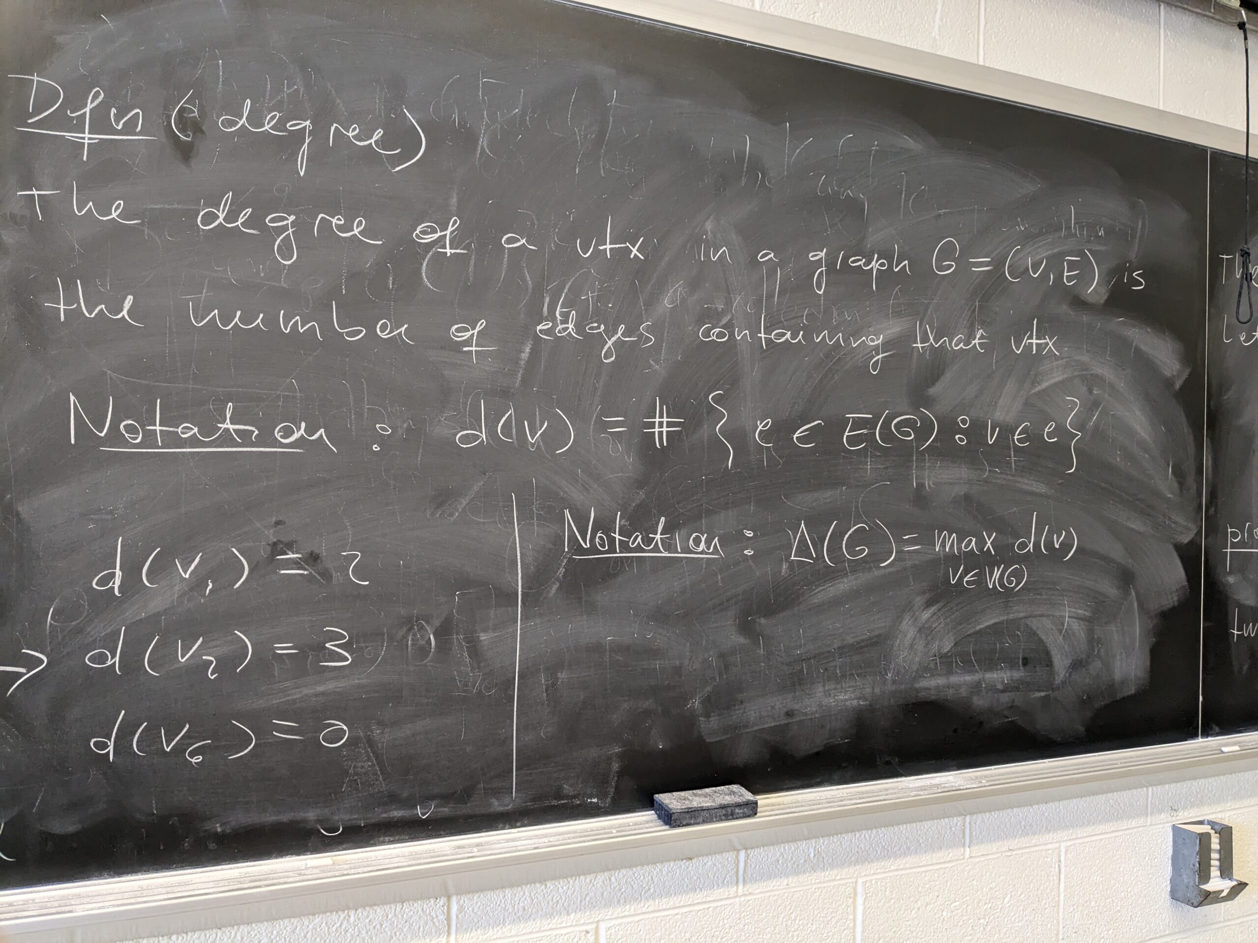
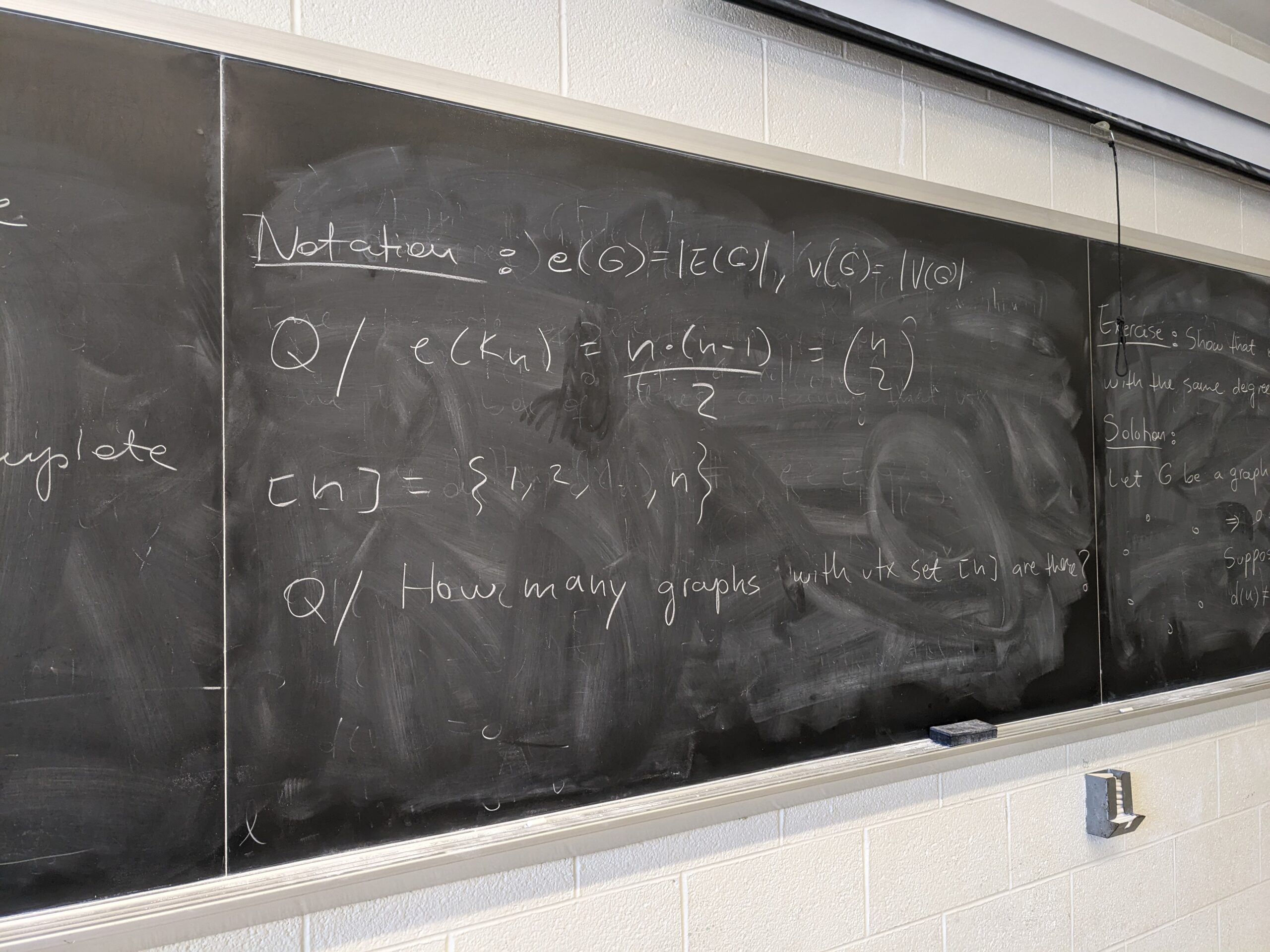
– Definition of degree and notation
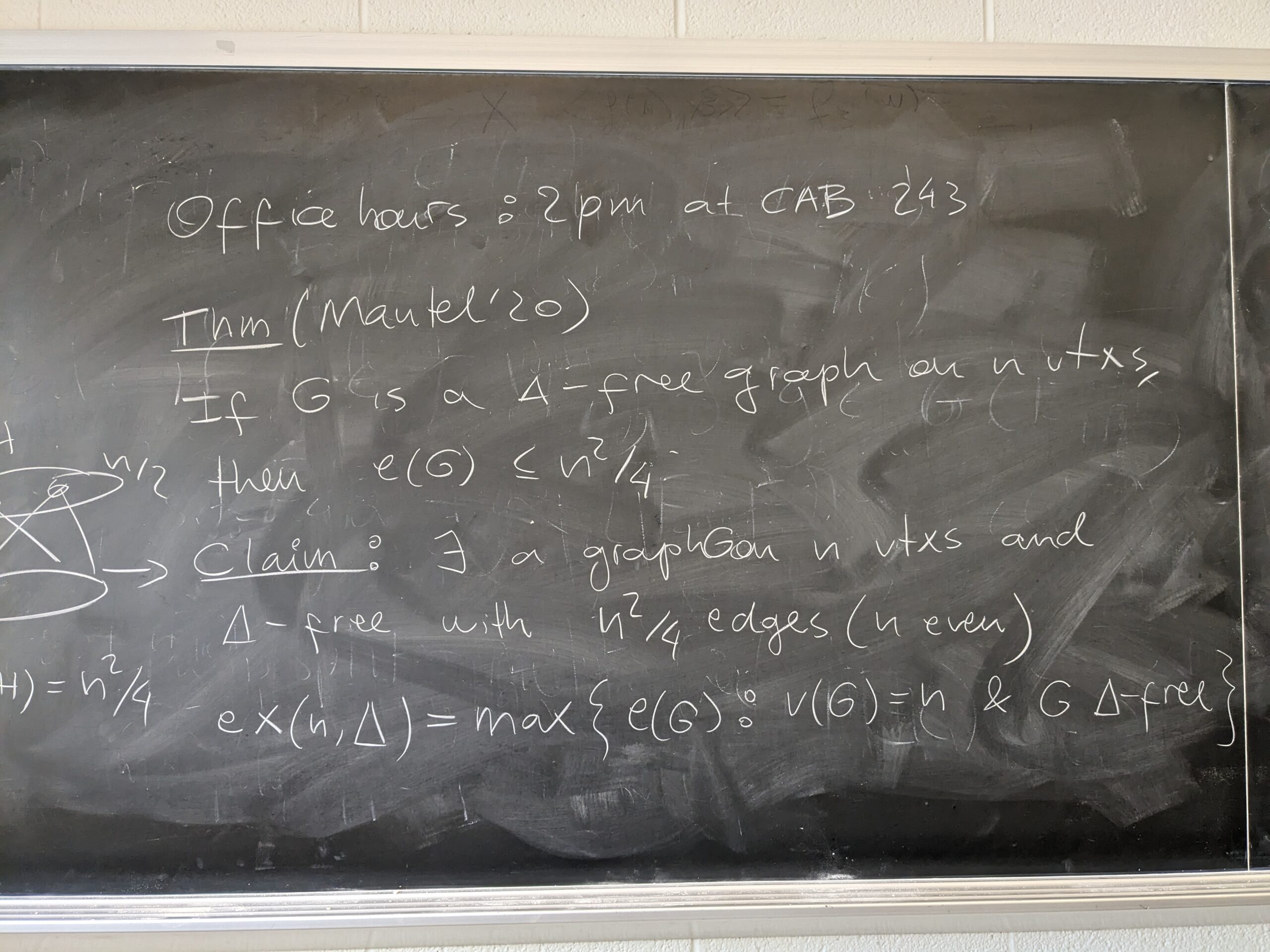
– The handshaking lemma
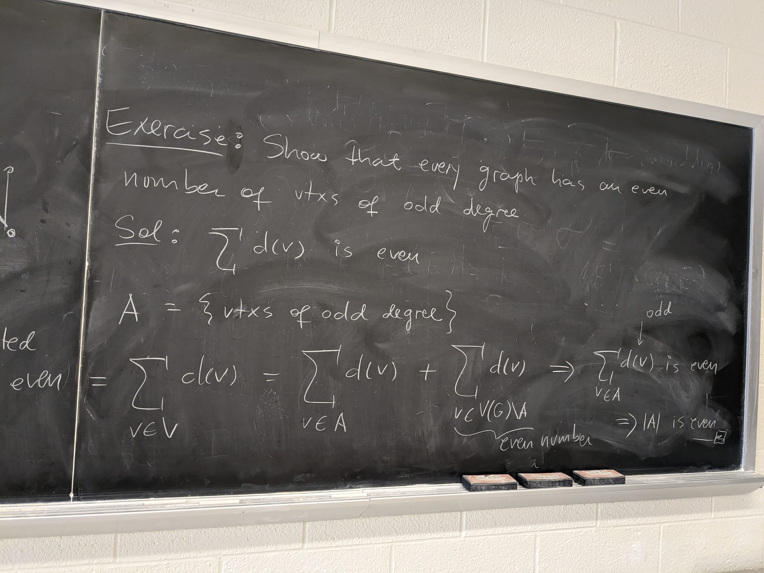
– Every graph has an even number of vertices of odd degree
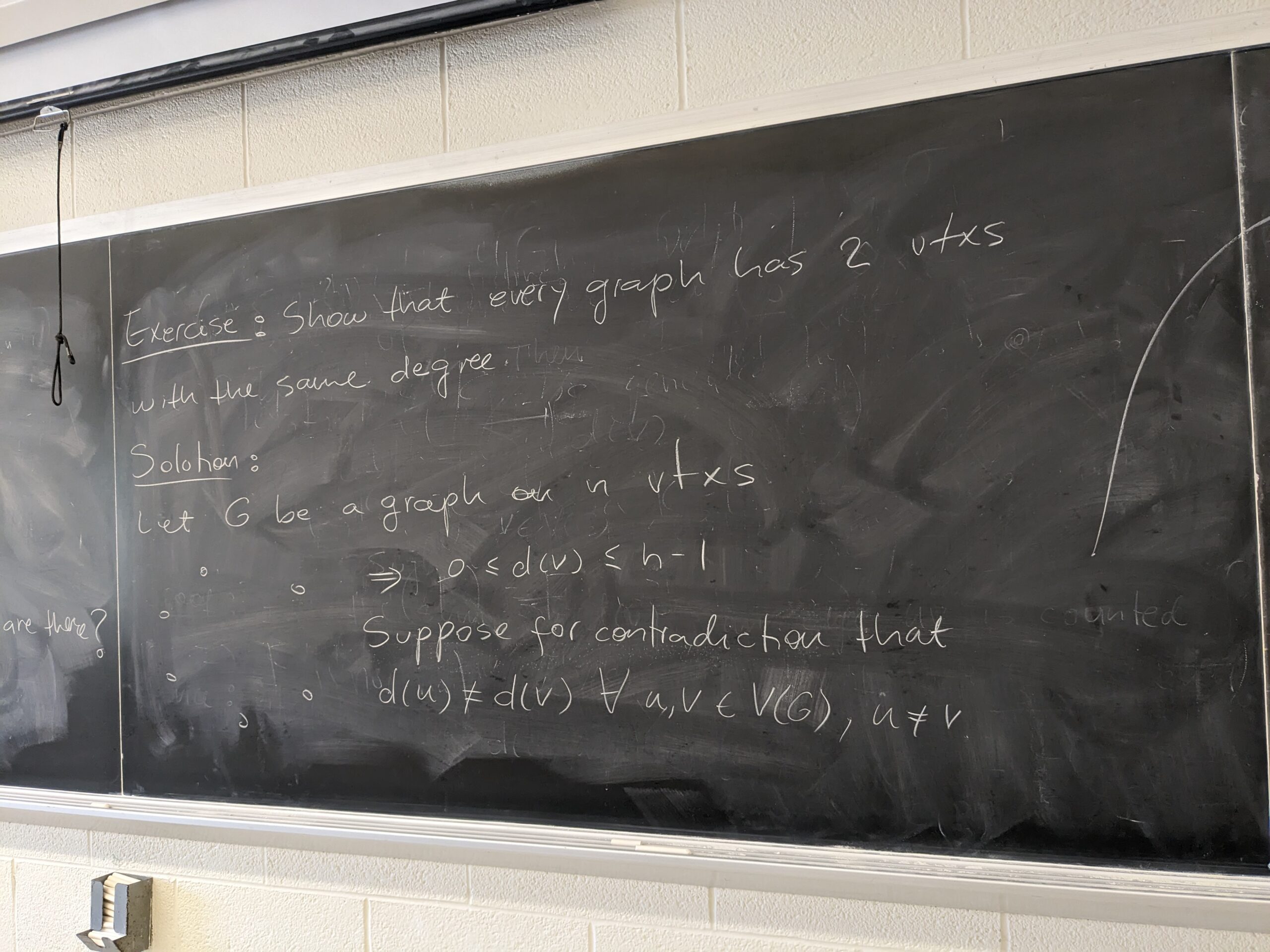
– Every graph has two vertices of same degree
– Definition of clique (complete graph)
– The number of graphs with vertex set \{1,2,\ldots,n\} is 2^{\binom{n}{2}}
– Proof of Mantel’s theorem. See Theorem 1 in these notes.
See some of the board pictures here: 1, 2, 3, 4, 5, 6, 7 and 8.
Lecture 38
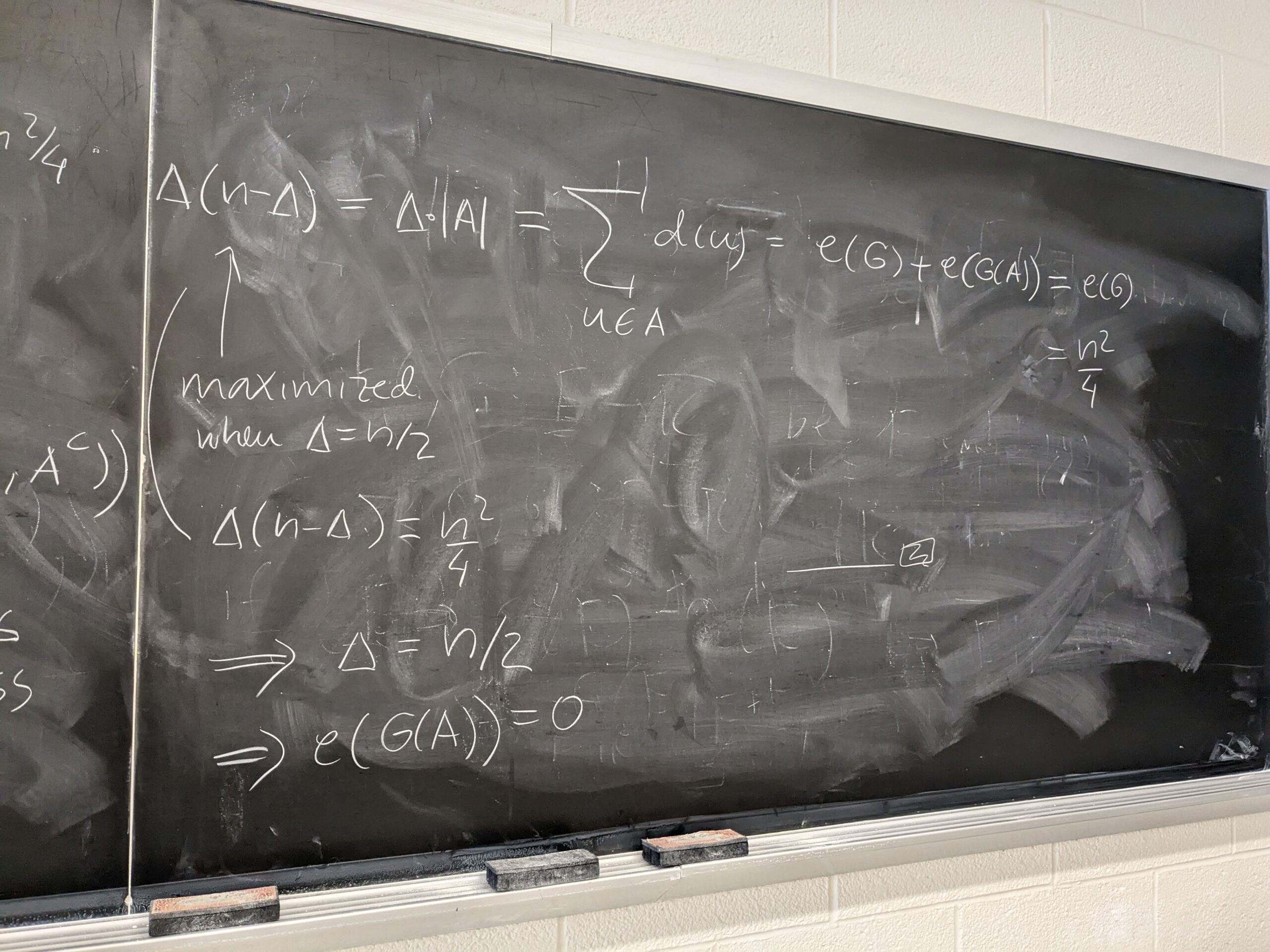
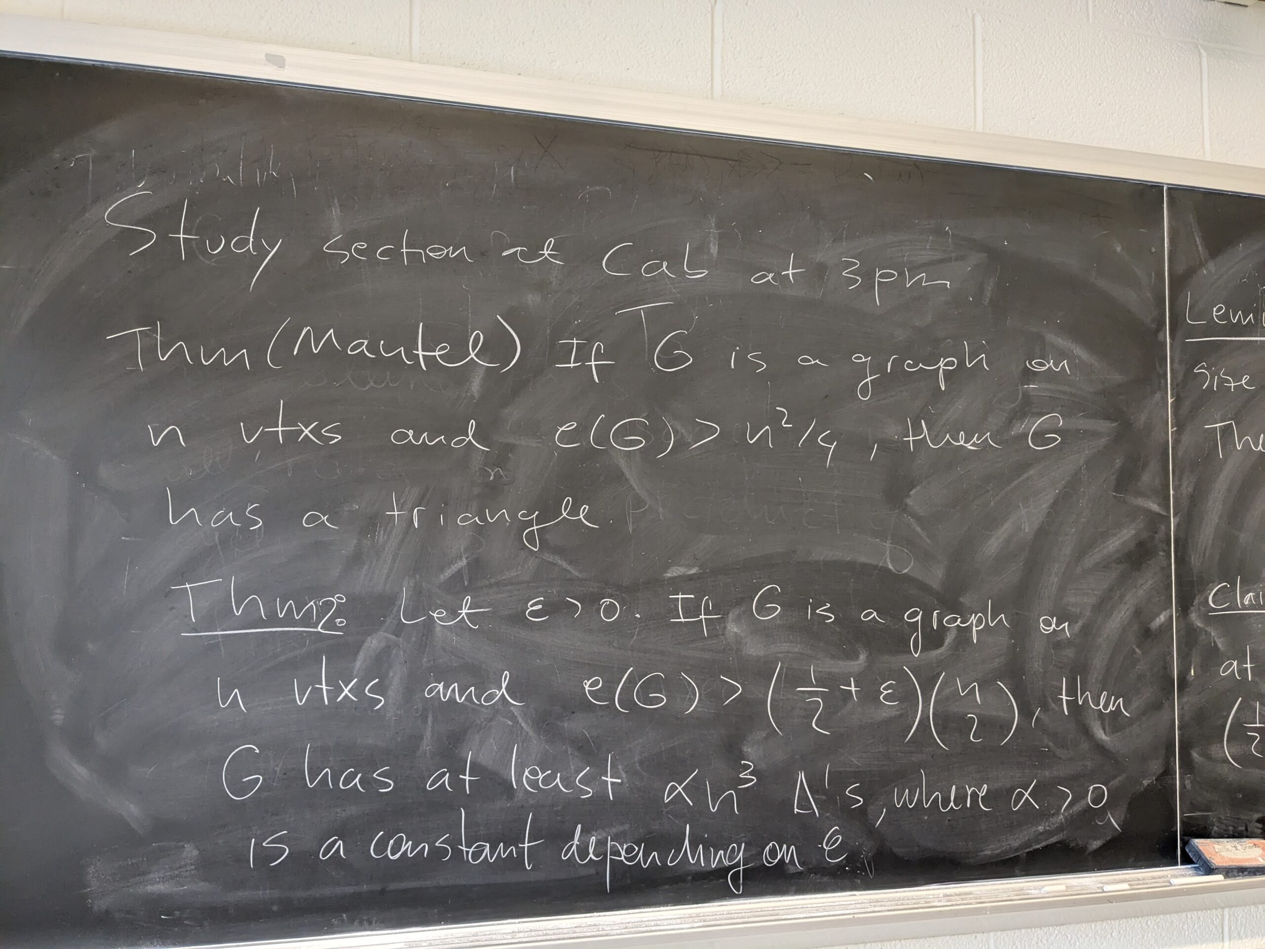
– Definition of \text{ex}(n,K_3) (the extremal number of the triangle)
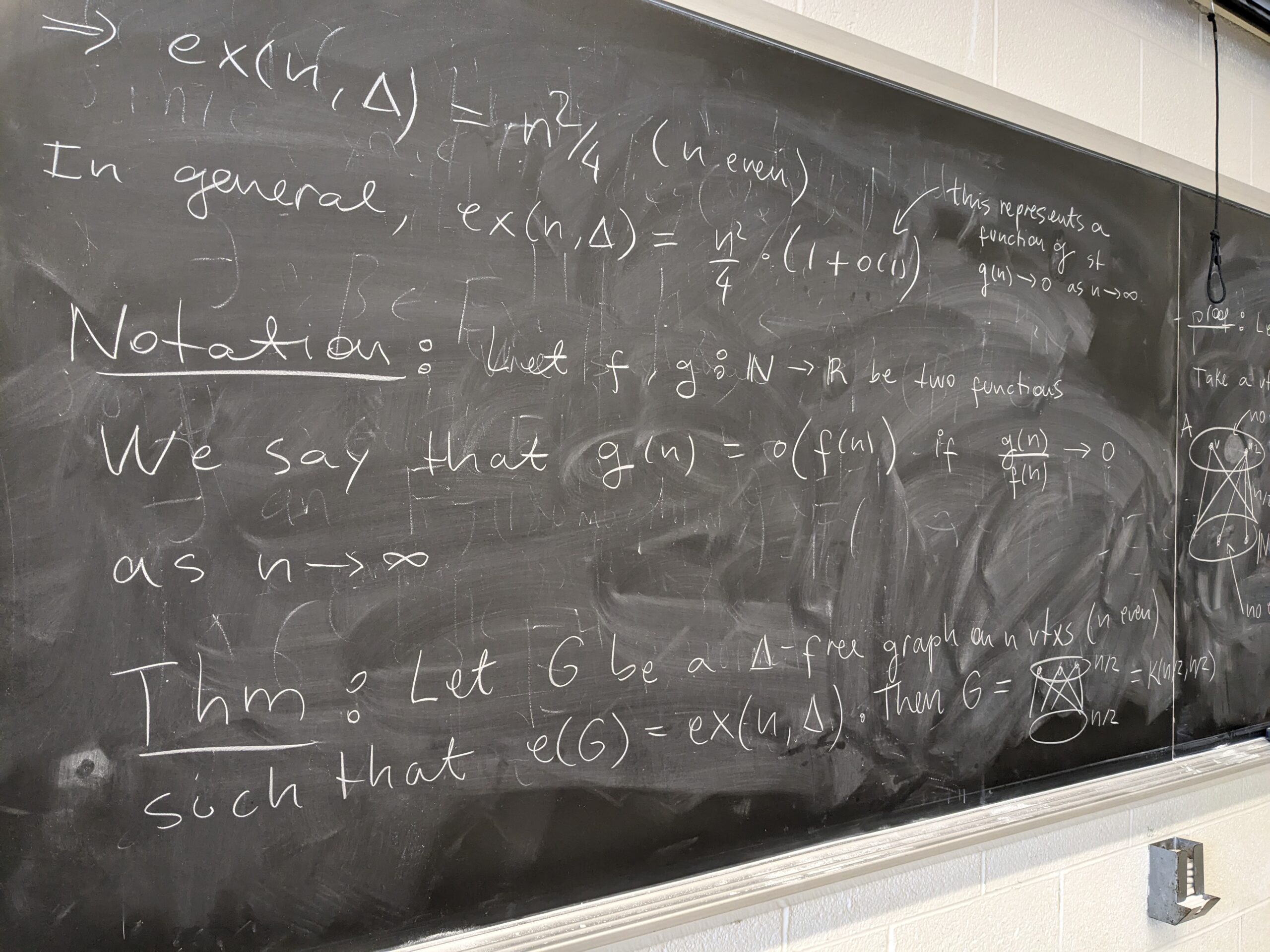
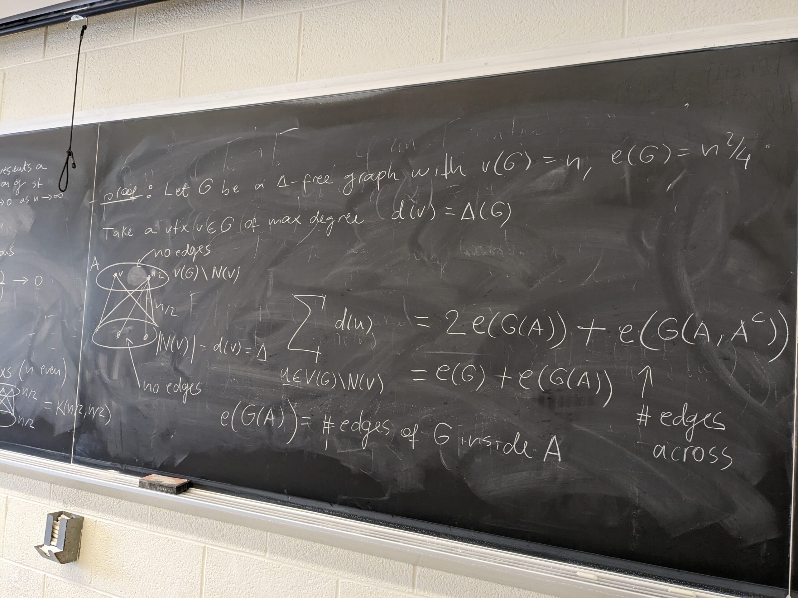
– Mantel’s theorem revisited: if G is a triangle-free graph on n vertices and e(G) = \text{ex}(n,K_3), then latex]G[/latex] is a complete bipartite graph, with parts of size \lfloor n/2 \rfloor and \lceil n/2 \rceil.
– Notation: G(S) denotes the graph with vertex set S and edge set \{T \subseteq S: T \in E(G)\}.
– Big Oh and little oh notation (see here, for example)
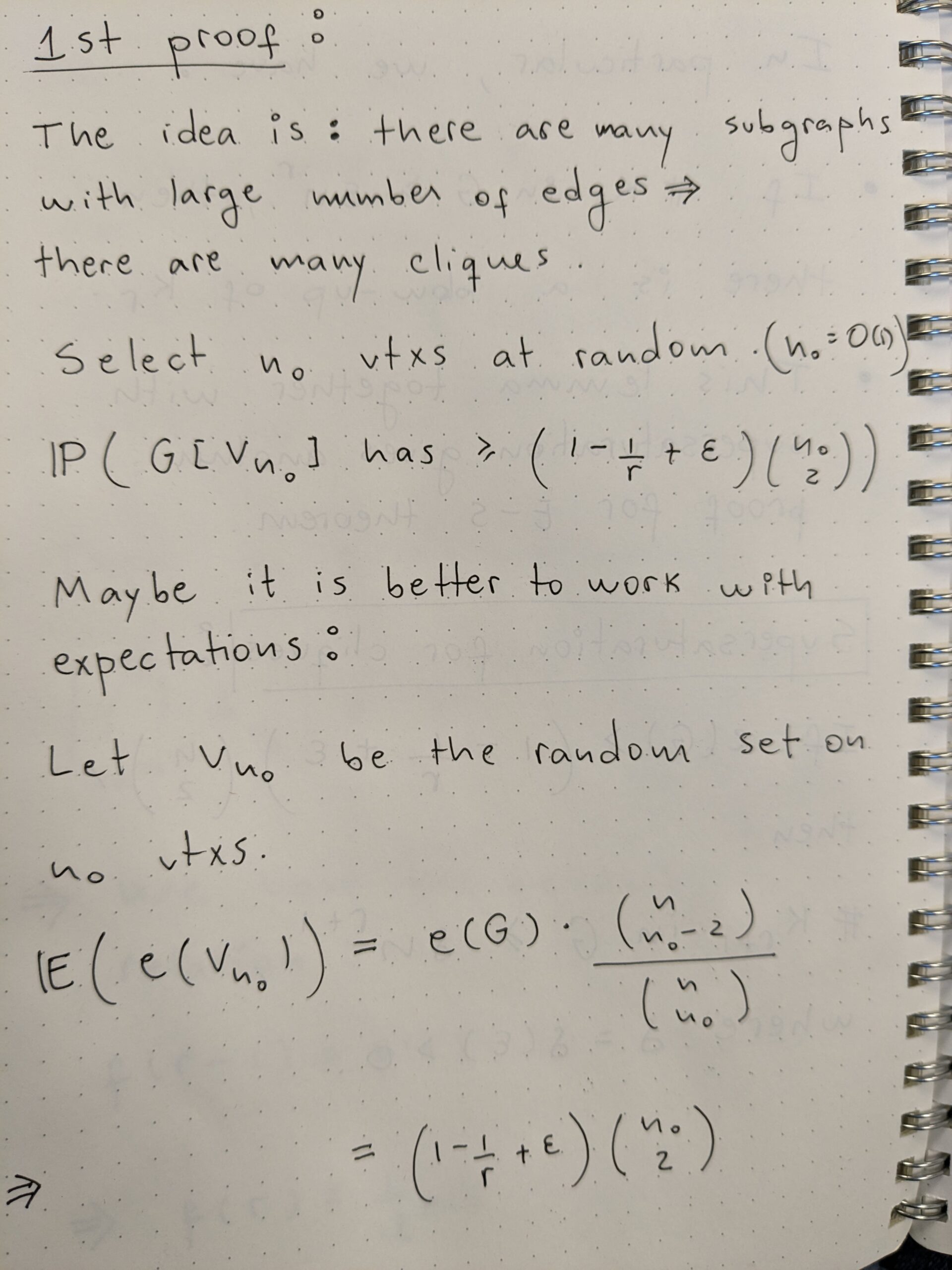
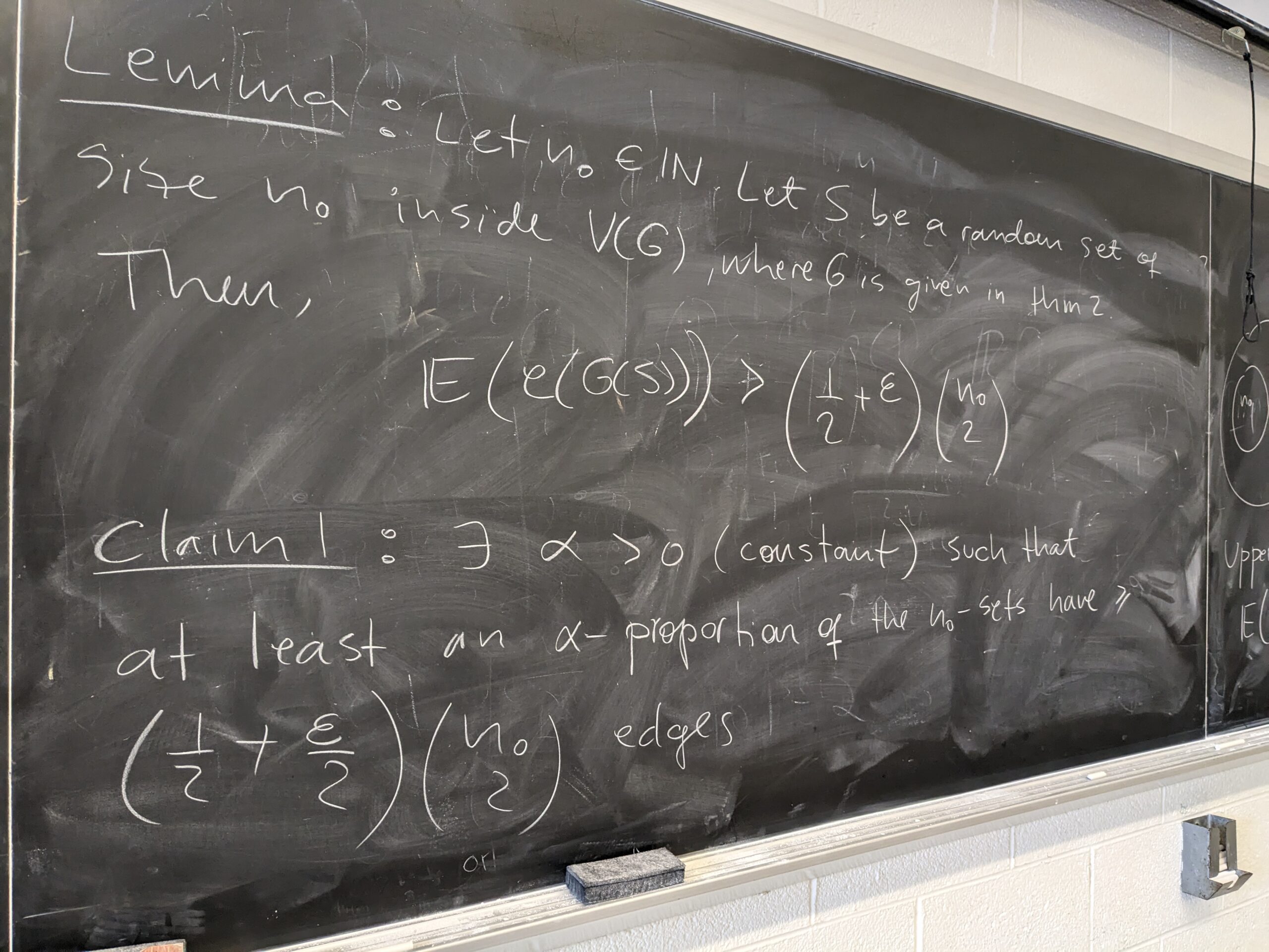
– Lemma: Let G be a graph on n vertices and at least \left (\frac{1}{2} + \varepsilon \right) \binom{n}{2} edges, where \varepsilon > 0 . Let S be a random uniformly-chosen set in V(G) of size n_0. Then, we have \mathbb{E}(e(G(S))) \ge \left (\frac{1}{2} + \varepsilon \right) \binom{n_0}{2}
– See a few board pictures (1, 2, 3 and 4) and my notes (1, 2, 3 and 4 — here r=2)
Lecture 39
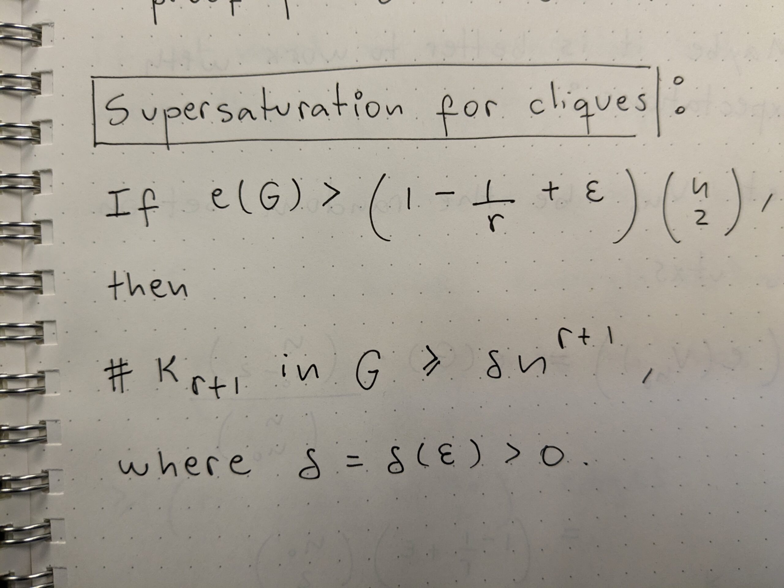
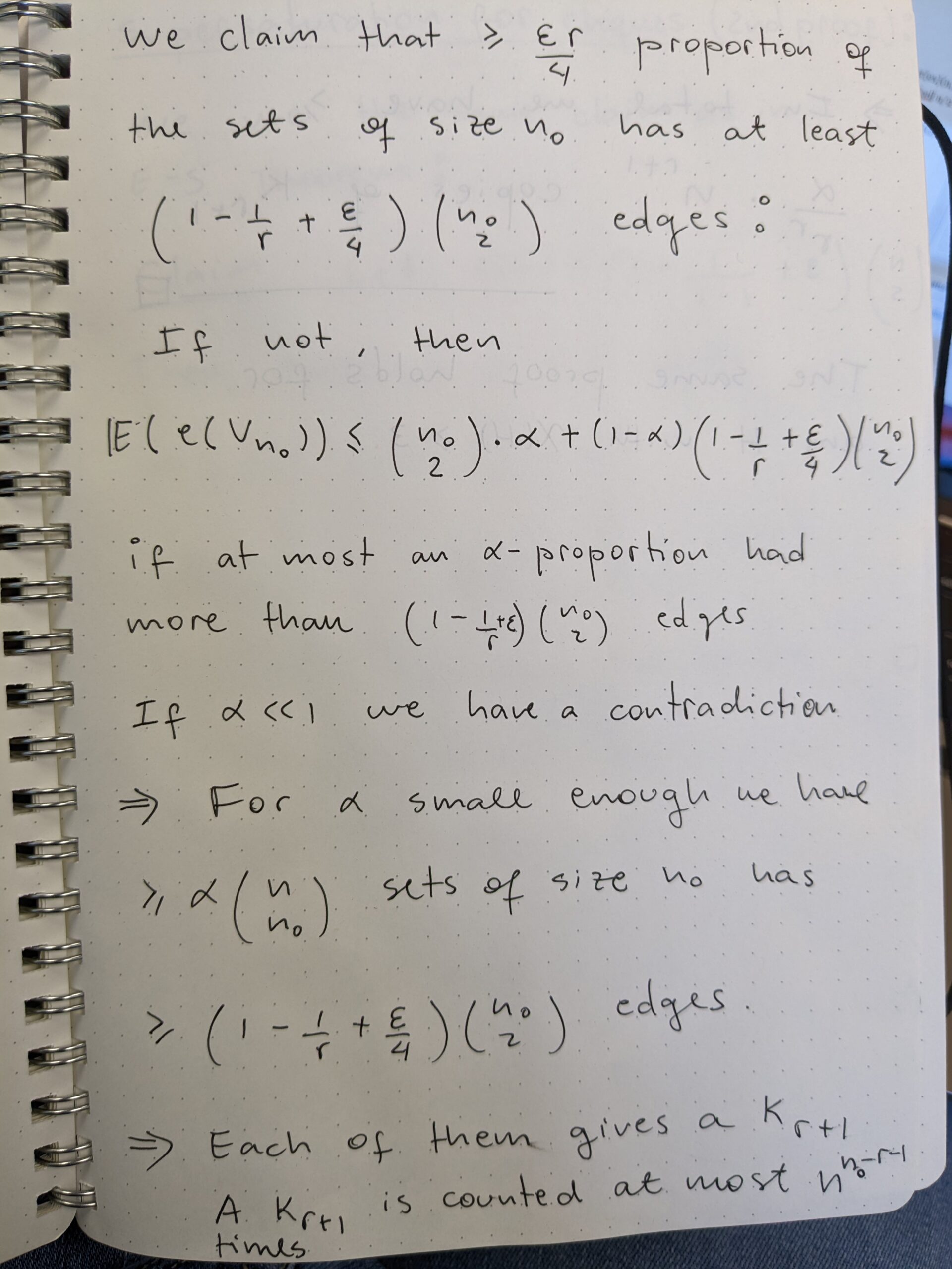
– Proof of the supersaturation theorem for triangles: if e(G)\ge \left (\frac{1}{2} + \varepsilon \right) \binom{n}{2} , then G has at least \alpha n^3 triangles, where \alpha>0 is a constant depending on \varepsilon.
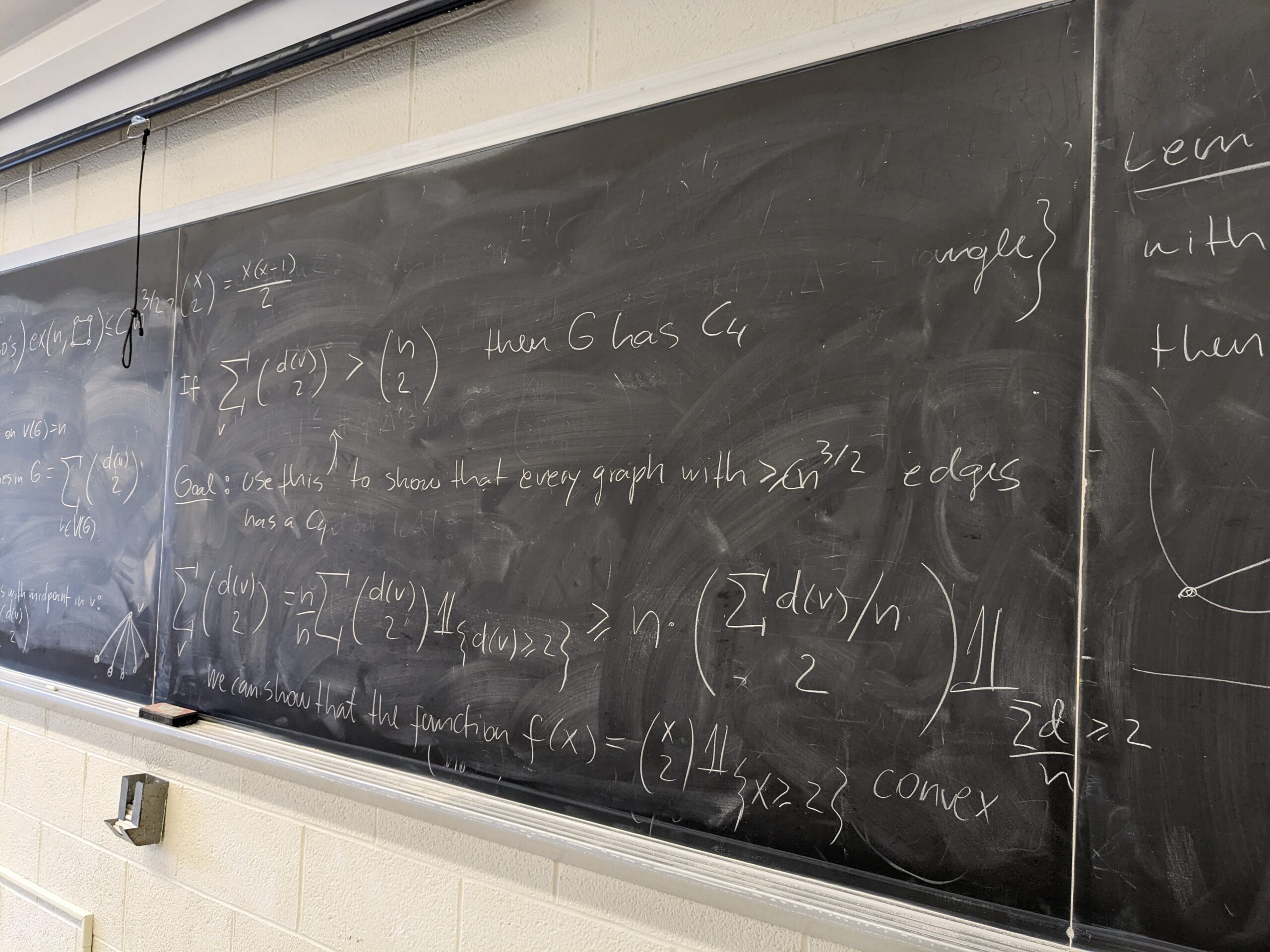
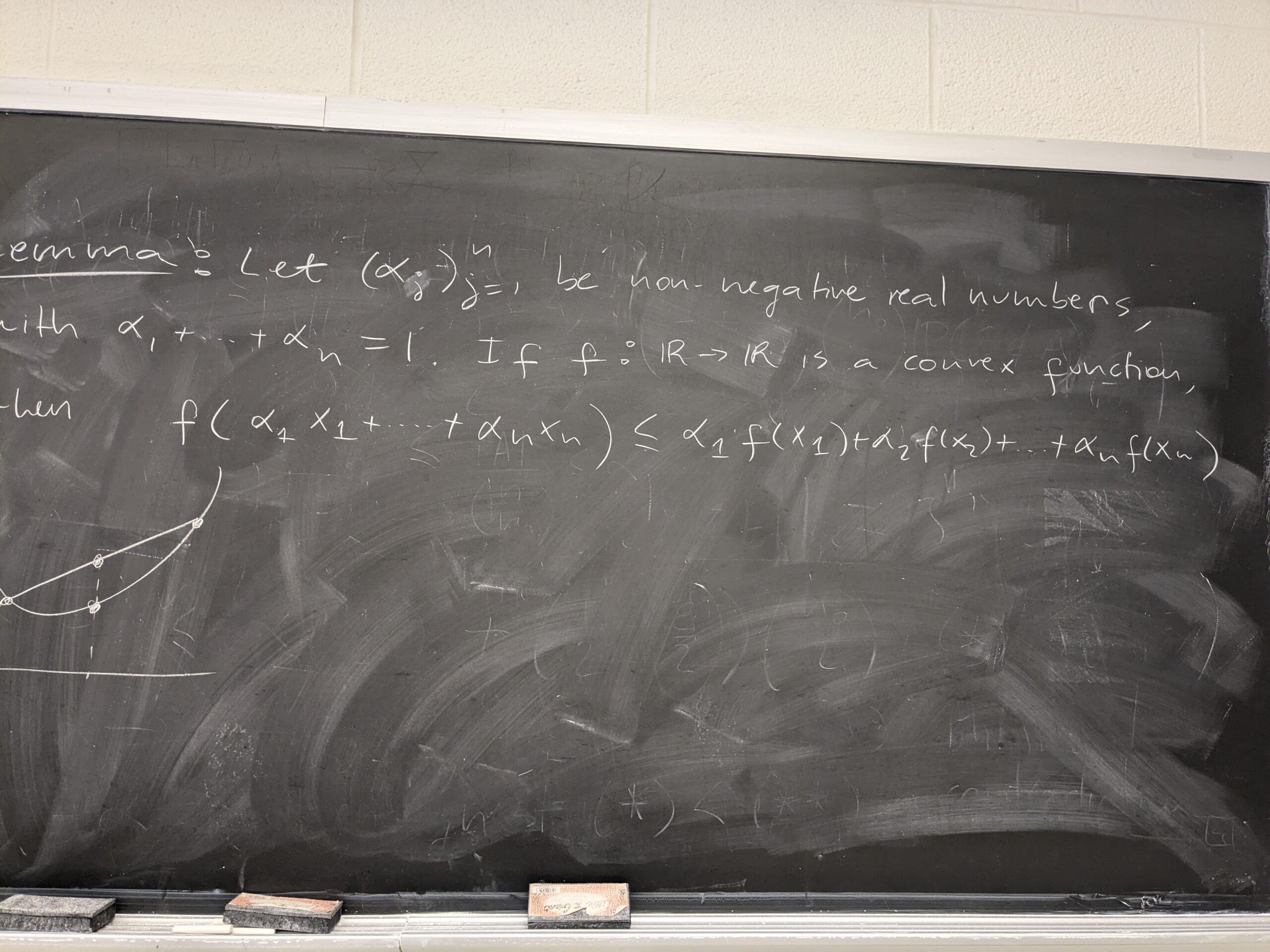
– Jensen’s inequality for convex functions
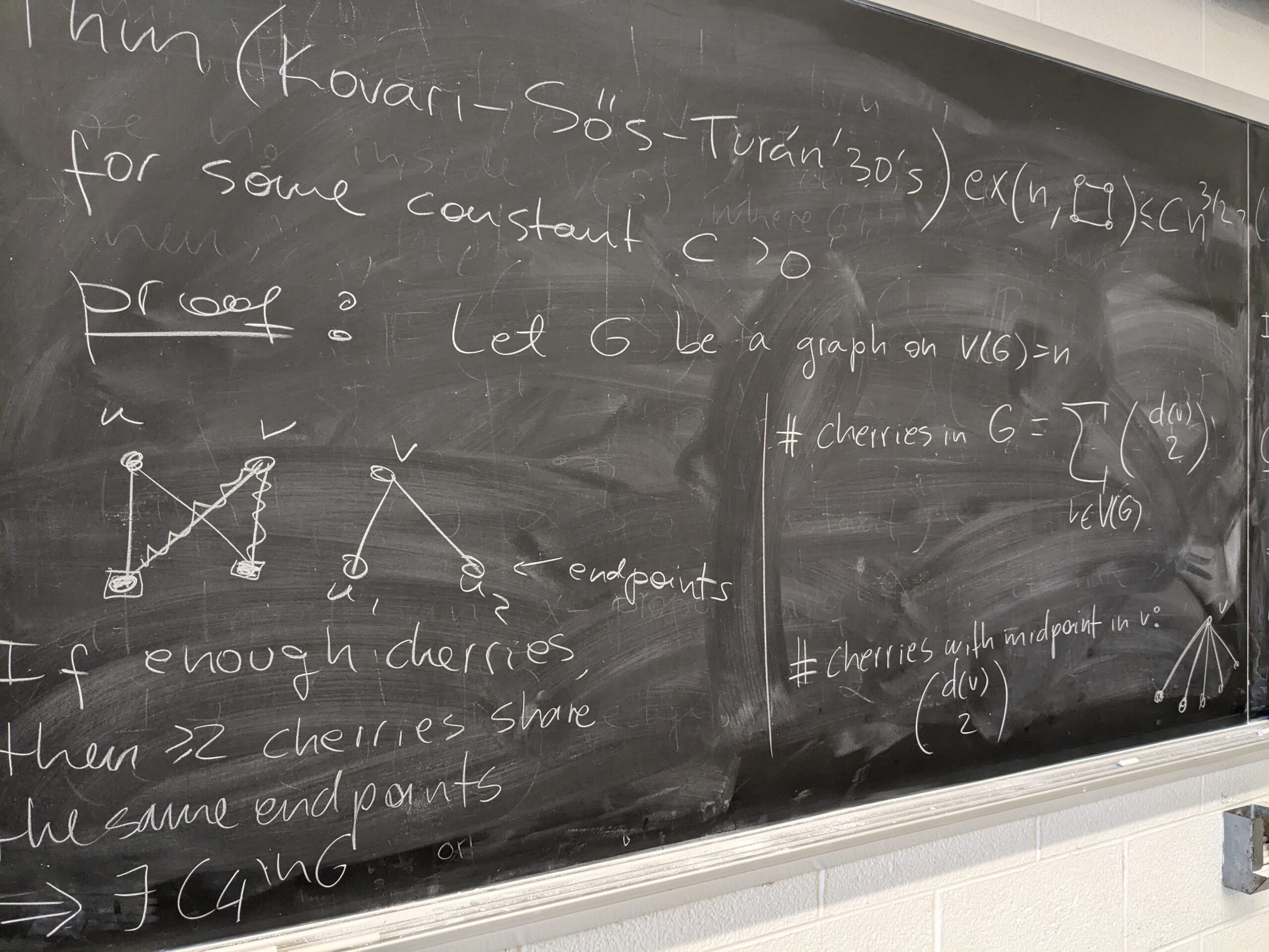
– Kovari–Sos–Turan theorem (for C4). See Theorem 3.1 in these notes
– See a few board pictures here: 1, 2, 3, 4, 5, 6, 7 and 8.
Lecture 40
– Finishing the proof of Kovari–Sos–Turan for C4
– Reviewing the content of the final exam